Page 390 - Schaum's Outline of Theory and Problems of Signals and Systems

CHAP. 71 STATE SPACE ANALYSIS 377

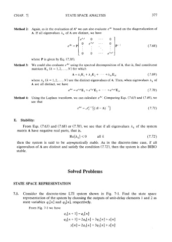
Method 2: Again, as in the evaluation of An we can also evaluate eA' based on the diagonalization of
A. If all eigenvalues A, of A are distinct, we have

eA' = P

where P is given by Eq. (7.30).
Method 3: We could also evaluate eA' using the spectral decomposition of A, that is, find constituent
matrices E, (k = 1,2,. . . , N) for which
A=A,El + A2E2 + ... +ANEN ( 7.69)

where A, (k = 1,2,. . . , N) are the distinct eigenvalues of A. Then, when eigenvalues A, of
A are all distinct, we have
.
+
.
eAt = eA~'El + eA~'~, . +eAN'E, (7.70)
Method 4: Using the Laplace transform, we can calculate eA'. Comparing Eqs. (7.63) and (7.49), we
see that

E. Stability:
From Eqs. (7.63) and (7.68) or (7.70), we see that if all eigenvalues A, of the system
matrix A have negative real parts, that is,
Re{A,) < 0 all k (7.72)

then the system is said to be asymptotically stable. As in the discrete-time case, if all
eigenvalues of A are distinct and satisfy the condition (7.721, then the system is also BIB0
stable.

Solved Problems

STATE SPACE REPRESENTATION

7.1. Consider the discrete-time LTI system shown in Fig. 7-1. Find the state space
representation of the system by choosing the outputs of unit-delay elements 1 and 2 as
state variables q,[n] and q2[n], respectively.

From Fig. 7-1 we have
41b + 11 =42M
42[n + 11 = 2q,[nl+ 3q2bI +xbI

ybI= 2q,[nl+ 3qhI +xbI