Page 428 - Schaum's Outline of Theory and Problems of Signals and Systems

CHAP. 71 STATE SPACE ANALYSIS 415

7.48. Using the state variables method, solve the second-order linear differential equation

y"(t) + 5y'(t) + 6y(t) =x(t) (7.127)
with the initial conditions y(0) = 2, yl(0) = 1, and x(t) = e-'u(t) (Prob. 3.38).
Let the state variables qJt) and q,(t) be

qdt) =Y(I) ~2( =~'(t)
)
f
Then the state space representation of Eq. (7.127) is given by [Eq. (7.19)l
q(t) = Aq(t) + bx(t)

~tt) =cq(t)
A=[-: -:I q'ol = [q2(0)] = [i]
with b=[y] c=[l O] qdo)

Thus, by Eq. (7.65)

with d = 0. Now, from the result from Prob. 7.39

-:I +e-''[-: -:I)[:]
and c~q(0) [I ~](e-~'[-:
=

Thus,

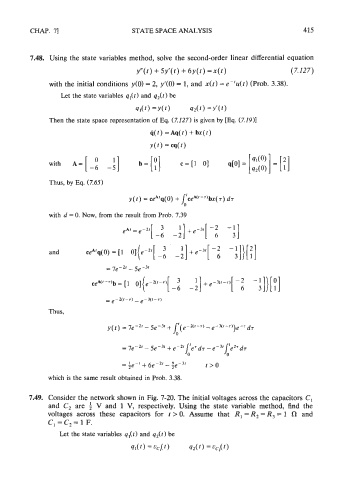
7.49. Consider the network shown in Fig. 7-20. The initial voltages across the capacitors C,
and C, are f V and 1 V, respectively. Using the state variable method, find the
voltages across these capacitors for t > 0. Assume that R, = R, = R, = 1 0 and
1
C, =C2= F.
Let the state variables q,(t) and q2( t) be