Page 429 - Schaum's Outline of Theory and Problems of Signals and Systems

STATE SPACE ANALYSIS [CHAP. 7

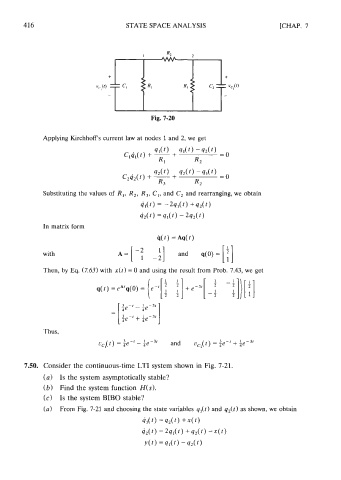
Fig. 7-20

Applying Kirchhoffs current law at nodes 1 and 2, we get

Substituting the values of R,, R2, R,, C,, and C2 and rearranging, we obtain
41(t) = -291(t) +q2(t)

42(t) =9l(t) -292(t)
In matrix form
il(t) =Aq(t)

with

Then, by Eq. (7.63) with x(t) = 0 and using the result from Prob. 7.43, we get

7.50. Consider the continuous-time LTI system shown in Fig. 7-21.
(a) Is the system asymptotically stable?
(b) Find the system function H(s).
(c) IS the system BIB0 stable?
(a) From Fig. 7-21 and choosing the state variables q,(t) and q2(t) as shown, we obtain
41(t) =92(t) +x(t)

42(t) = 29l(t) +92(t) -x(t)
~(t) 9Lt) - %(t)
=