Page 68 - Schaum's Outline of Theory and Problems of Signals and Systems

CHAP. 21 LINEAR TIME-INVARIANT SYSTEMS 5 7

Equation (2.5) indicates that a continuous-time LTI system is completely characterized by
its impulse response h( t 1.

C. Convolution Integral:
Equation (2.5) defines the convolution of two continuous-time signals x(t) and h(t)
denoted by

Equation (2.6) is commonly called the convolution integral. Thus, we have the fundamental
result that the output of any continuous-time LTI system is the convolution of the input x(t)
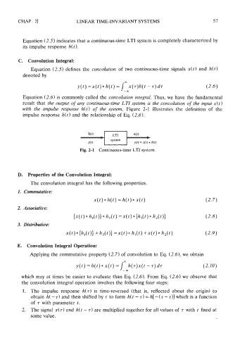
with the impulse response h(t) of the system. Figure 2-1 illustrates the definition of the
impulse response h(t) and the relationship of Eq. (2.6).

Fig. 2-1 Continuous-time LTl system.

D. Properties of the Convolution Integral:
The convolution integral has the following properties.

I. Commutative:
*
~(t) h(t) = h(t) * ~(t)
2. Associative:
*
{xP) * hl(4 * h,(t) = x(t) * {hl(f) h2(4
3. Distributive:

x(t) * {h,(t)) +hN =x(t) * hl(t) +x(t) * h,(t)

E. Convolution Integral Operation:

Applying the commutative property (2.7) of convolution to Eq. (2.61, we obtain
00
(t) = h ) * x ) = h(r)x(t - r) dr (2.10)
- m
which may at times be easier to evaluate than Eq. (2.6). From Eq. (2.6) we observe that
the convolution integral operation involves the following four steps:

is
1. The impulse response h(~) time-reversed (that is, reflected about the origin) to
obtain h( -7) and then shifted by t to form h(t - r) = h[-(r - t)] which is a function
of T with parameter t.
2. The signal x(r) and h(t - r) are multiplied together for all values of r with t fixed at
some value.