Page 73 - Schaum's Outline of Theory and Problems of Signals and Systems

62 LINEAR TIME-INVARIANT SYSTEMS [CHAP. 2

B. Response to an Arbitrary Input:
From Eq. ( 1.51) the input x[n] can be expressed as

Since the system is linear, the response y[n] of the system to an arbitrary input x[n] can be
expressed as

= x[k]T{S[n - k]}

Since the system is time-invariant, we have
h[n - k] = T{S[n - k]) (2.33)
Substituting Eq. (2.33) into Eq. (2.321, we obtain
x
Y [ ~ I C x[klh[n - kl
=
k= -m
Equation (2.34) indicates that a discrete-time LTI system is completely characterized by its
impulse response h[n].

C. Convolution Sum:
Equation (2.34) defines the convolution of two sequences x[n] and h[n] denoted by

Equation (2.35) is commonly called the con~~olution sum. Thus, again, we have the
fundamental result that the output of any discrete-time LTI system is the concolution of the
input x[n] with the impulse response h[n] of the system.
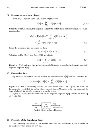
Figure 2-3 illustrates the definition of the impulse response h[n] and the relationship
of Eq. (2.35).

614 ~n hlnl
).
system
xlnl vlnl= x[nl* hlnj
Fig. 2-3 Discrete-time LTI system.

D. Properties of the Convolution Sum:
The following properties of the convolution sum are analogous to the convolution
integral properties shown in Sec. 2.3.