Page 72 - Schaum's Outline of Theory and Problems of Signals and Systems

CHAP. 21 LINEAR TIME-INVARIANT SYSTEMS

Y,(O
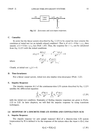
Fig. 2-2 Zero-state and zero-input responses.

C. Causality:
In order for the linear system described by Eq. (2.25) to be causal we must assume the
condition of initial rest (or an initially relaxed condition). That is, if x( t) = 0 for t I t,,, then
assume y(t) = 0 for t 5 to (see Prob. 1.43). Thus, the response for t > to can be calculated
from Eq. (2.25) with the initial conditions

where

Clearly, at initial rest y,,(t) = 0.

D. Time-Invariance:
For a linear causal system, initial rest also implies time-invariance (Prob. 2.22).

E. Impulse Response:
The impulse response h(t) of the continuous-time LTI system described by Eq. (2.25)
satisfies the differential equation

with the initial rest condition. Examples of finding impulse responses are given in Probs.
2.23 to 2.25. In later chapters, we will find the impulse response by using transform
techniques.

2.6 RESPONSE OF A DISCRETE-TIME LTI SYSTEM AND CONVOLUTION SUM
A. Impulse Response:

The impulse response (or unit sample response) h[n] of a discrete-time LTI system
(represented by T) is defined to be the response of the system when the input is 6[n], that
is,