Page 138 - Schaum's Outlines - Probability, Random Variables And Random Processes

CHAP. 4) FUNCTIONS OF RANDOM VARIABLES, EXPECTATION, LIMIT THEOREMS 131

(a) (b)
Fig. 4-2
(b) Find the pdf of Y in terms of fx(x).
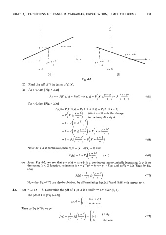
(a) If a > 0, then [Fig. 4-2(a)]
f &) = P(Y 6 y) = P(aX + b i y) = P(X 5 q)
Fx($)
=
If a < 0, then [Fig. 4-2(b)]
F&) = P(Y S y) = P(aX + b 6 y) = P(aX I - b)
y
(since a < 0, note the change
=P(Xze) in the inequality sign)

-1-P(X<?)
= 1 - P(X.5) + P(X +)

= 1 - Fx(e) + f'(x = E$)

Note that if X is continuous, then P[X = (y - b)/a] = 0, and

(b) From Fig. 4-2, we see that y = g(x) = ax + b is a contirluous monotonically increasing (a > 0) or
decreasing (a < 0) function. Its inverse is x = g-'(y) = h(y) = (y - b)/a, and dx/dy = l/a. Thus, by Eq.
(4.61,

Note that Eq. (4.70) can also be obtained by differentiating Eqs. (4.67) and (4.69) with respect to y.

4.4. Let Y = ax + b. Determine the pdf of Y, if X is a uniform r.v. over (0, 1).
The pdf of X is [Eq. (2.44)]
1 O<x<l
fx(x) = {O
otherwise
Then by Eq. (4.70), we get
I
1
YERY
otherwise