Page 237 - Schaum's Outlines - Probability, Random Variables And Random Processes

ANALYSIS AND PROCESSING OF RANDOM PROCESSES [CHAP 6

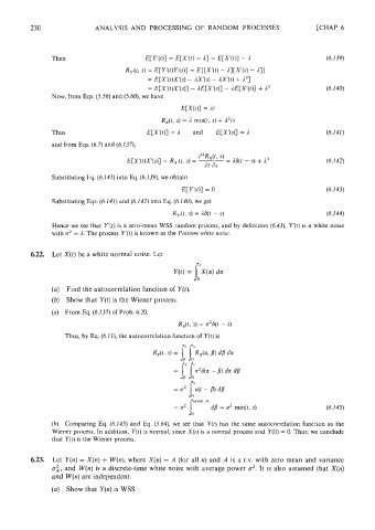
Then
Ry*(t, S) = E[Yf(t)Yf(s)] = E{[X1(t) - L][Xf(s) - I])
= E[Xf(t)Xr(s) - LX1(s) - IXr(t) + 12]
= E [Xr(t)X1(s)] - LE[Xf(s)] - IEIX1(t)] + L2
Now, from Eqs. (5.56) and (5.60), we have

Thus EIX1(t)] = A and E[Xr(s)] = 1 (6.1 41)
and from Eqs. (6.7) and (6.137),

Substituting Eq. (6.1 41) into Eq. (6.1 39), we obtain

Substituting Eqs. (6.141) and (6.142) into Eq. (6.140), we get

Hence we see that Y1(t) is a zero-mean WSS random process, and by definition (6.43), Y'(t) is a white noise
with a2 = I. The process Y1(t) is known as the Poisson white noise.

6.22. Let X(t) be a white normal noise. Let

(a) Find the autocorrelation function of Y(t).
(b) Show that Y(t) is the Wiener process.

(a) From Eq. (6.1 37) of Prob. 6.20,

Thus, by Eq. (6.1 l), the autocorrelation function of Y(t) is

(b) Comparing Eq. (6.145) and Eq. (5.64), we see that Y(t) has the same autocorrelation function as the
Wiener process. In addition, Y(t) is normal, since X(t) is a normal process and Y(0) = 0. Thus, we conclude
that Y(t) is the Wiener process.

6.23. Let Y(n) = X(n) + W(n), where X(n) = A (for all n) and A is a r.v. with zero mean and variance
a:, and W(n) is a discrete-time white noise with average power a2. It is also assumed that X(n)
and W(n) are independent.
(a) Show that Y(n) is WSS.