Page 58 - Schaum's Outlines - Probability, Random Variables And Random Processes

CHAP. 21 RANDOM VARIABLES

Again using Eq. (2.10), we obtain
P(a < X < b) = P(a < X I b) - P(X = b)
= Fx(b) - Fx(a) - P(X = b)
Similarly, P(a I X I b) = P[(a I X < b) u (X = b)]
= P(a I X < b) + P(X = b)
Using Eq. (2.64), we obtain
P(a I X < b) = P(a 5 X 5 b) - P(X = b)
= P(X = a) + Fx(b) - F,(a) - P(X = b)

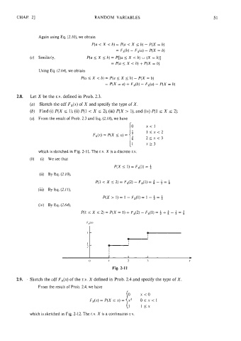
X be the r.v. defined in Prob. 2.3.
Sketch the cdf FX(x) of X and specify the type of X.
Find (i) P(X I I), (ii) P(l < X I 2), (iii) P(X > I), and (iv) P(l I X I 2).
From the result of Prob. 2.3 and Eq. (2.18), we have

which is sketched in Fig. 2-1 1. The r.v. X is a discrete r.v.
(i) We see that
P(X 5 1) = Fx(l) = 4
(ii) By Eq. (2.1 O),

P(l < X 5 2) = Fx(2) - FA1) = - 4 =
(iii) By Eq. (2.1 I),
P(X > 1) = 1 - Fx(l) = 1 - $ = $

(iv) By Eq. (2.64),
P(l I X I 2) = P(X = 1) + Fx(2) - Fx(l) = 3 + 3 - 3 = 3

Fig. 2-1 1

Sketch the cdf F,(x) of the r.v. X defined in Prob. 2.4 and specify the type of X.
From the result of Prob. 2.4, we have
0 x<o
FX(x)=P(XIx)=
1 llx
which is sketched in Fig. 2-12. The r.v. X is a continuous r.v.