Page 158 - Semiconductor For Micro- and Nanotechnology An Introduction For Engineers

Basic Equations of Electrodynamics
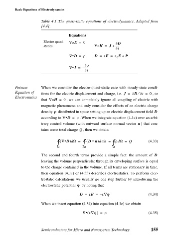
Table 4.1. The quasi-static equations of electrodynamics. Adapted from
[4.4].
Equations
Electro-quasi- ∇× E = 0 ∂D
statics ∇× H = J +
t ∂
∇• D = ρ D = εE = ε E + P
0
∂ρ
∇• J = –
t ∂

Poisson When we consider the electro-quasi-static case with steady-state condi-
Equation of tions for the electric displacement and charge, i.e. J = ∂D ∂t = 0 , so
⁄
Electrostatics
that ∇× H = 0 , we can completely ignore all coupling of electric with
magnetic phenomena and only consider the effects of an electric charge
ρ
density distributed in space setting up an electric displacement field D
according to ∇• D = ρ . When we integrate equation (4.1c) over an arbi-
trary control volume (with outward surface normal vector ) that con-
n
tains some total charge Q , then we obtain

∫
∫
∫ ( ∇• D) Ω = ° ( Dn)d Ω = ° ρΩ = Q (4.33)
∂
•
d
d
°
Ω ∂ Ω Ω
The second and fourth terms provide a simple fact: the amount of D
leaving the volume perpendicular through its enveloping surface is equal
to the charge contained in the volume. If all terms are stationary in time,
then equation (4.1c) or (4.33) describes electrostatics. To perform elec-
trostatic calculations we usually go one step further by introducing the
ψ
electrostatic potential by noting that
D = εE = ε – ∇ ψ (4.34)

When we insert equation (4.34) into equation (4.1c) we obtain

∇
∇• ( εψ) = ρ (4.35)

Semiconductors for Micro and Nanosystem Technology 155