Page 182 - Semiconductor For Micro- and Nanotechnology An Introduction For Engineers

Particle Statistics: Counting Particles
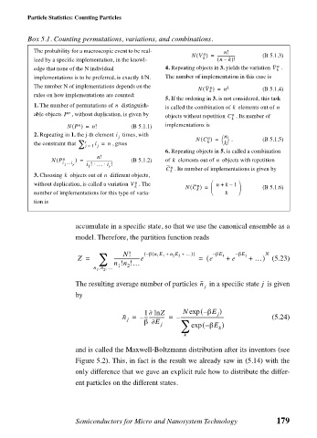
Box 5.1. Counting permutations, variations, and combinations.
The probability for a macroscopic event to be real- n!
n
(
NV ) = ------------------ (B 5.1.3)
–
ized by a specific implementation, in the knowl- k ( nk)!
edge that none of the N individual 4. Repeating objects in 3. yields the variation V k n .
implementations is to be preferred, is exactly 1/N. The number of implementation in this case is
The number N of implementations depends on the n k
(
NV k ) = n (B 5.1.4)
rules on how implementations are counted:
5. If the ordering in 3. is not considered, this task
n
1. The number of permutations of distinguish- is called the combination of elements out of n
k
able objects P n , without duplication, is given by objects without repetition C n . Its number of
k
(
n
NP ) = n! (B 5.1.1) implementations is
i
2. Repeating in 1. the j-th element times, with NC ) = n  . (B 5.1.5)
j
n
(
the constraint that ∑ r j = 1 i = n , gives k k 
j
6. Repeating objects in 5. is called a combination
n!
(
NP n ) = -------------------------- (B 5.1.2) of elements out of objects with repetition
n
k
i …i
1 r i ! … i !⋅ ⋅ r n
1
C k . Its number of implementations is given by
k
n
3. Choosing objects out of different objects,
without duplication, is called a variation V n k . The NC k ) =   n + k – 1   (B 5.1.6)
n
(
number of implementations for this type of varia-  k 
tion is
accumulate in a specific state, so that we use the canonical ensemble as a
model. Therefore, the partition function reads
N!
(
∑ ---------------------e – ( β n 1 E 1 + n 2 E 2 + …)) e ( – βE 1 – βE 2 …) N
Z = n !n !… = + e + (5.23)
n 1 n 2 …, , 1 2
The resulting average number of particles n in a specific state is given
j
j
by
∂
1 lnZ N exp – ( βE )
j
n = – ---------------- = – ----------------------------------- (5.24)
j
∂
β E j ∑ exp – ( βE )
k
k
and is called the Maxwell-Boltzmann distribution after its inventors (see
Figure 5.2). This, in fact is the result we already saw in (5.14) with the
only difference that we gave an explicit rule how to distribute the differ-
ent particles on the different states.
Semiconductors for Micro and Nanosystem Technology 179