Page 218 - Sensing, Intelligence, Motion : How Robots and Humans Move in an Unstructured World

PLANAR REVOLUTE–REVOLUTE (RR) ARM 193

2. One degree of freedom of the system (not necessarily one arm link) is con-
strained by an obstacle boundary; then only points along the virtual line—that
is, a one-dimensional curve—are available for the next positions of the arm
endpoint.
3. Two degrees of freedom of the system are constrained: No motion is possible.

Because of our model’s assumption that some motion is always possible, case 3
is impossible. Case 2 thus includes all cases of interaction between the arm and
obstacles.

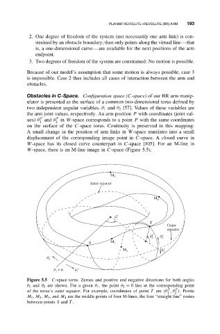
Obstacles in C-Space. Configuration space (C-space) of our RR arm manip-
ulator is presented as the surface of a common two-dimensional torus defined by
two independent angular variables, θ 1 and θ 2 [57]. Values of these variables are
the arm joint values, respectively. An arm position P with coordinates (joint val-
p p
ues) θ and θ in W-space corresponds to a point P with the same coordinates
1 2
on the surface of the C-space torus. Continuity is preserved in this mapping:
A small change in the position of arm links in W-space translates into a small
displacement of the corresponding image point in C-space. A closed curve in
W-space has its closed curve counterpart in C-space [105]. For an M-line in
W-space, there is an M-line image in C-space (Figure 5.5).

M 3
Inner equator

M 4

T
q 1
T
Outer
equator
q T 2 q + 2
S M 1
−
M 2 q 2
q 1 −

q = 0 q 1 +
1
Figure 5.5 C-space torus. Zeroes and positive and negative directions for both angles
θ 1 and θ 2 are shown. For a given θ 1 , the point θ 2 = 0 lies at the corresponding point
T
T
of the torus’s outer equator. For example, coordinates of point T are (θ ,θ ). Points
1 2
M 1 ,M 2 ,M 3 ,and M 4 are the middle points of four M-lines, the four “straight line” routes
between points S and T .