Page 221 - Sensing, Intelligence, Motion : How Robots and Humans Move in an Unstructured World

196 MOTION PLANNING FOR TWO-DIMENSIONAL ARM MANIPULATORS

17
16
B
18
15

S
1
19
24 8
7 14
9 2
H 1
3
23 6 13
5
4
22 10
A
21 20
11 L 1
12
T
q 1 = 0
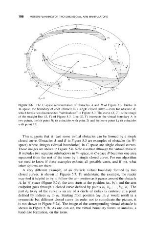
Figure 5.6 The C-space representation of obstacles A and B of Figure 5.3. Unlike in
W-space, the boundary of each obstacle is a single closed curve—even for obstacle B,
which forms two disconnected “subshadows” in Figure 5.3. The curve (S, T ) is the image
of the straight line (S, T ) of Figure 5.3. Line (S, T ) intersects the virtual boundary A in
two points, the hit point H 1 (it coincides with point 2) and the leave point L 1 (it coincides
with point 12).

This suggests that at least some virtual obstacles can be formed by a single
closed curve. Obstacles A and B in Figure 5.3 are examples of obstacles (in W-
space) whose images (virtual boundaries) in C-space are single closed curves.
Those images are shown in Figure 5.6. Note also that although the virtual obstacle
B includes two separate subshadows in W-space, in C-space B becomes one area
separated from the rest of the torus by a single closed curve. For our algorithm
we need to know if these examples exhaust all possible cases, and if not, what
other options are there.
A very different example, of an obstacle virtual boundary formed by two
closed curves, is shown in Figures 5.7. To understand the example, the reader
may find it helpful to try to follow the arm motion as it passes around the obstacle
A.In W-space (Figure 5.7a), the arm starts at the position (a 1 ,b 1 ), and the arm
endpoint goes through a closed curve defined by points b 1 ,b 2 ,...,b 10 ,b 1 .The
part b 4 to b 8 of the curve is an arc of a circle of radius l 2 centered at a point
defined by indices a 4 to a 8 . Starting from position (a 11 ,b 11 ) would result in a
symmetric but different closed curve (in order not to complicate the picture, it
is not shown in Figure 5.7a). The image of the corresponding virtual obstacle is
shown in Figure 5.7b. As one can see, the virtual boundary forms an annulus, a
band-like formation, on the torus.