Page 225 - Sensing, Intelligence, Motion : How Robots and Humans Move in an Unstructured World

200 MOTION PLANNING FOR TWO-DIMENSIONAL ARM MANIPULATORS

q = 0
2

b
l 2
J 1
a
q 2 q
l 1 1
A
q = 0
J o 1
O

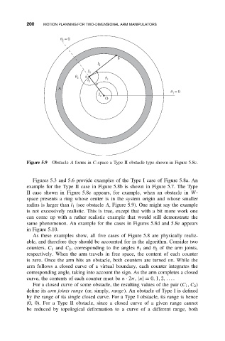
Figure 5.9 Obstacle A forms in C-space a Type II obstacle type shown in Figure 5.8c.

Figures 5.3 and 5.6 provide examples of the Type I case of Figure 5.8a. An
example for the Type II case in Figure 5.8b is shown in Figure 5.7. The Type
II case shown in Figure 5.8c appears, for example, when an obstacle in W-
space presents a ring whose center is in the system origin and whose smaller
radius is larger than l 1 (see obstacle A, Figure 5.9). One might say the example
is not excessively realistic. This is true, except that with a bit more work one
can come up with a rather realistic example that would still demonstrate the
same phenomenon. An example for the cases in Figures 5.8d and 5.8e appears
in Figure 5.10.
As these examples show, all five cases of Figure 5.8 are physically realiz-
able, and therefore they should be accounted for in the algorithm. Consider two
counters, C 1 and C 2 , corresponding to the angles θ 1 and θ 2 of the arm joints,
respectively. When the arm travels in free space, the content of each counter
is zero. Once the arm hits an obstacle, both counters are turned on. While the
arm follows a closed curve of a virtual boundary, each counter integrates the
corresponding angle, taking into account the sign. As the arm completes a closed
curve, the contents of each counter must be n · 2π, |n|= 0, 1, 2,... .
For a closed curve of some obstacle, the resulting values of the pair (C 1 ,C 2 )
define its arm joints range (or, simply, range). An obstacle of Type I is defined
by the range of its single closed curve. For a Type I obstacle, its range is hence
(0, 0). For a Type II obstacle, since a closed curve of a given range cannot
be reduced by topological deformation to a curve of a different range, both