Page 72 - Sensing, Intelligence, Motion : How Robots and Humans Move in an Unstructured World

TRAJECTORY MODIFICATION 47

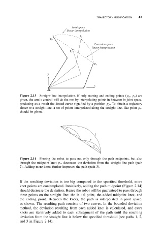
Joint space
linear interpolation
p j
p b
Cartesian space
linear interpolation
p c

p a

y

x

Figure 2.13 Straight-line interpolation. If only starting and ending points (p a , p b )are
given, the arm’s control will do the rest by interpolating points in between in joint space,
producing as a result the dotted curve signified by a position p j . To obtain a trajectory
closer to a straight line, a set of points interpolated along the straight line, like point p c ,
should be given.

1
2
3

Figure 2.14 Forcing the robot to pass not only through the path endpoints, but also
through the midpoint knot p c , decreases the deviation from the straight-line path (path
2). Adding more knots further improves the path (path 3).

If the resulting deviation is too big compared to the specified threshold, more
knot points are contemplated. Intuitively, adding the path midpoint (Figure 2.14)
should decrease the deviation. Hence the robot will be guaranteed to pass through
three points on the straight line: the initial point, the added midpoint knot, and
the ending point. Between the knots, the path is interpolated in joint space,
as shown. The resulting path consists of two curves. In the bounded deviation
method, the deviation resulting from each added knot is calculated, and extra
knots are iteratively added to each subsegment of the path until the resulting
deviation from the straight line is below the specified threshold (see paths 1, 2,
and 3 in Figure 2.14).