Page 70 - Sensing, Intelligence, Motion : How Robots and Humans Move in an Unstructured World

TRAJECTORY MODIFICATION 45

p b

p a

q 2

q 1

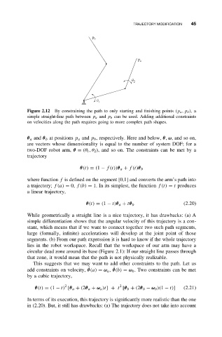
Figure 2.12 By constraining the path to only starting and finishing points (p a ,p b ),a
simple straight-line path between p a and p b can be used. Adding additional constraints
on velocities along the path requires going to more complex path shapes.

θ a and θ b at positions p a and p b , respectively. Here and below, θ, ω, and so on,
are vectors whose dimensionality is equal to the number of system DOF; for a
two-DOF robot arm, θ = (θ 1 ,θ 2 ), and so on. The constraints can be met by a
trajectory

θ(t) = (1 − f(t))θ a + f(t)θ b

where function f is defined on the segment [0,1] and converts the arm’s path into
a trajectory; f(a) = 0, f(b) = 1. In its simplest, the function f(t) = t produces
a linear trajectory,

θ(t) = (1 − t)θ a + tθ b (2.20)

While geometrically a straight line is a nice trajectory, it has drawbacks: (a) A
simple differentiation shows that the angular velocity of this trajectory is a con-
stant, which means that if we want to connect together two such path segments,
large (formally, infinite) accelerations will develop at the joint point of those
segments. (b) From our path expression it is hard to know if the whole trajectory
lies in the robot workspace. Recall that the workspace of our arm may have a
circular dead zone around its base (Figure 2.1): If our straight line passes through
that zone, it would mean that the path is not physically realizable.
This suggests that we may want to add other constraints to the path. Let us
add constraints on velocity, θ(a) = ω a , θ(b) = ω b . Two constraints can be met
˙
˙
by a cubic trajectory,
2 2
θ(t) = (1 − t) [θ a + (2θ a + ω a )t] + t [θ b + (2θ b − ω b )(1 − t)] (2.21)

In terms of its execution, this trajectory is significantly more realistic than the one
in (2.20). But, it still has drawbacks: (a) The trajectory does not take into account