Page 564 - Sensors and Control Systems in Manufacturing

0.07 SpectRx NIR Technology 517
0.06
Radiometric accuracy 0.04 3.5 mm
0.05
2 mm

0.03

0.02
0.01 5 mm
0
375 575 775 975 1175 1375 1575 1775
Temperature of the scene (K)
–1
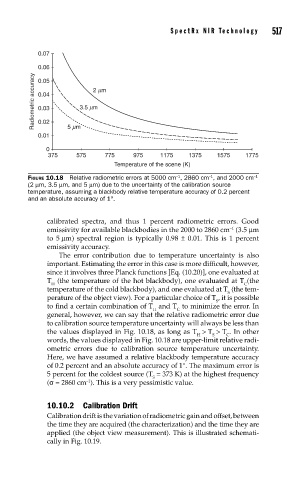
FIGURE 10.18 Relative radiometric errors at 5000 cm , 2860 cm , and 2000 cm
–1
–1
(2 μm, 3.5 μm, and 5 μm) due to the uncertainty of the calibration source
temperature, assuming a blackbody relative temperature accuracy of 0.2 percent
and an absolute accuracy of 1°.
calibrated spectra, and thus 1 percent radiometric errors. Good
emissivity for available blackbodies in the 2000 to 2860 cm (3.5 μm
–1
to 5 μm) spectral region is typically 0.98 ± 0.01. This is 1 percent
emissivity accuracy.
The error contribution due to temperature uncertainty is also
important. Estimating the error in this case is more difficult, however,
since it involves three Planck functions [Eq. (10.20)], one evaluated at
T (the temperature of the hot blackbody), one evaluated at T (the
H C
temperature of the cold blackbody), and one evaluated at T (the tem-
S
perature of the object view). For a particular choice of T , it is possible
S
to find a certain combination of T and T to minimize the error. In
H C
general, however, we can say that the relative radiometric error due
to calibration source temperature uncertainty will always be less than
the values displayed in Fig. 10.18, as long as T > T > T . In other
H S C
words, the values displayed in Fig. 10.18 are upper-limit relative radi-
ometric errors due to calibration source temperature uncertainty.
Here, we have assumed a relative blackbody temperature accuracy
of 0.2 percent and an absolute accuracy of 1°. The maximum error is
5 percent for the coldest source (T = 373 K) at the highest frequency
S
(σ = 2860 cm ). This is a very pessimistic value.
–1
10.10.2 Calibration Drift
Calibration drift is the variation of radiometric gain and offset, between
the time they are acquired (the characterization) and the time they are
applied (the object view measurement). This is illustrated schemati-
cally in Fig. 10.19.