Page 190 - Separation process engineering

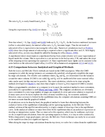
(4-65)

The ratio L /V is easily found from L /D as
0
1
0

Using this expression in Eq. (4-65) we obtain

(4-66)

Note that when f = 0, Eqs. (4-65) and (4-66) both say L /V = L /V . As the fraction condensed increases
1
1
c
2
0
(reflux is subcooled more), the internal reflux ratio, L /V , becomes larger. Thus the net result of
2
1
subcooled reflux is equivalent to increasing the reflux ratio. Numerical calculations (such as Problem
4.D5) show that a large amount of subcooling is required to have a significant effect on L/V. With highly
subcooled reflux, an extra tray should be added for heating the reflux (Kister, 1990).
A superheated direct steam input or a superheated boilup from a total reboiler will cause vaporization of
liquid inside the column. This is equivalent to a net increase in the boilup ratio, /B, and makes the slope
of the stripping section operating line approach 1.0. Since superheated vapor inputs can be analyzed in the
same fashion as the subcooled liquid reflux, it will be left as homework assignments 4.C14 and 4.C15.

4.15 Comparisons between Analytical and Graphical Methods

Both the Lewis and McCabe-Thiele methods are based on the CMO assumption. When the CMO
assumption is valid, the energy balances are automatically satisfied, which greatly simplifies the stage-
by-stage calculations. The reboiler and condenser duties, Q and Q , are determined from the balances
c
R
around the entire column. If CMO is not valid, Q and Q will be unaffected if the same external reflux
c
R
ratio can be used, but this may not be possible. The exact calculation, which can be done using the
methods developed in Chapter 6, may show that a higher or lower L /D is required if CMO is invalid.
0
When a programmable calculator or a computer is to be used, the analytical method is more convenient,
particularly if a spreadsheet is used (Burns and Sung, 1996). The computer calculations are obviously
more convenient if a very large number of stages are required, if a trial-and-error solution is required, or
if many cases are to be run to explore the effect of many variables (e.g., for economic analysis).
However, since accuracy is limited by the equilibrium data, the computer calculations assuming CMO are
not more accurate than the graphical method.

If calculations are to be done by hand, the graphical method is faster than alternating between the
analytical forms of the equilibrium relationship and the operating equations. In the McCabe-Thiele
method, solution of the equilibrium relationship is simply a matter of drawing a line to the equilibrium
curve. In the analytical solution we must first either fit the equilibrium data to an analytical expression or
develop an interpolation routine. Then we must solve this equation, which may be nonlinear, each time
we do an equilibrium calculation. Since the operating equation is linear, it is easy to solve analytically.
With a sharp pencil, large graph paper, and care, the McCabe-Thiele technique can easily be as accurate
as the equilibrium data (two significant figures).

When doing the stage-by-stage calculations from the top down, we solve for x values from the equilibrium