Page 200 - Six Sigma for electronics design and manufacturing

The Use of Six Sigma with High- and Low-Volume Products and Processes
167
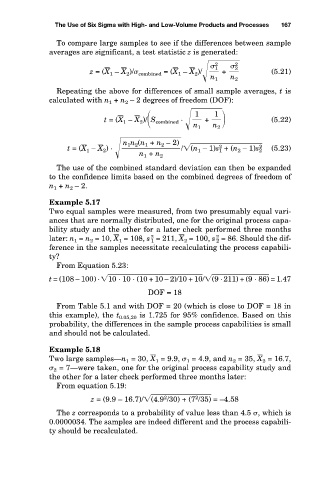
To compare large samples to see if the differences between sample
averages are significant, a test statistic z is generated:

2
2
2
1
z = (X 1 – X 2 )/ combined = (X 1 – X 2 )/
+
n 2
n 1
Repeating the above for differences of small sample averages, t is
calculated with n 1 + n 2 – 2 degrees of freedom (DOF):

1
1
t = (X 1 – X 2 )/ S combined ·
(5.22)
+

n 2
n 1
/ (n 1 – 1 )s 1 + ( n 2 – 1 )s 2 2 (5.21)
n 1 n 2 (n 1 + n 2 – 2)

2
t = (X 1 – X 2 )· (5.23)
n 1 + n 2
The use of the combined standard deviation can then be expanded
to the confidence limits based on the combined degrees of freedom of
n 1 + n 2 – 2.
Example 5.17
Two equal samples were measured, from two presumably equal vari-
ances that are normally distributed, one for the original process capa-
bility study and the other for a later check performed three months
2
2
later: n 1 = n 2 = 10, X 1 = 108, s 1 = 211, X 2 = 100, s 2 = 86. Should the dif-
ference in the samples necessitate recalculating the process capabili-
ty?
From Equation 5.23:
t = (108 – 100) · 1 0 · 1 0 · ( 1 0 + 1 0 – 2 )/ 1 0 + 1 0 / (9 · 2 1 1 ) + ( 9 · 8 6 ) = 1.47
DOF = 18
From Table 5.1 and with DOF = 20 (which is close to DOF = 18 in
this example), the t 0.05,20 is 1.725 for 95% confidence. Based on this
probability, the differences in the sample process capabilities is small
and should not be calculated.
Example 5.18
Two large samples—n 1 = 30, X 1 = 9.9, 1 = 4.9, and n 2 = 35, X 2 = 16.7,
2 = 7—were taken, one for the original process capability study and
the other for a later check performed three months later:
From equation 5.19:
2
2
z = (9.9 – 16.7)/ (4 .9 / 3 0 ) + ( 7 / 3 5 ) = –4.58
The z corresponds to a probability of value less than 4.5 , which is
0.0000034. The samples are indeed different and the process capabili-
ty should be recalculated.