Page 131 -

102 PART TWO MANAGING SOFTWARE PROJECTS

E r , errors found/review hour 3
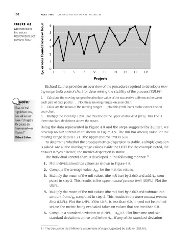
FIGURE 4.8 6
Metrics data
for errors 5
uncovered per
review hour 4

2
1

0
5
3
11
9
1
7
Projects 13 15 17 19
Richard Zultner provides an overview of the procedure required to develop a mov-
ing range (mR) control chart for determining the stability of the process [ZUL99]:
1. Calculate the moving ranges: the absolute value of the successive differences between
each pair of data points . . . Plot these moving ranges on your chart.
“If we can’t tell 2. Calculate the mean of the moving ranges . . . plot this (“mR bar”) as the center line on
signals from noise, your chart.
how will we ever 3. Multiply the mean by 3.268. Plot this line as the upper control limit [UCL]. This line is
know if changes to three standard deviations above the mean.
the process are
improvement—or Using the data represented in Figure 4.8 and the steps suggested by Zultner, we
illusions?” develop an mR control chart shown in Figure 4.9. The mR bar (mean) value for the
Richard Zultner moving range data is 1.71. The upper control limit is 5.58.
To determine whether the process metrics dispersion is stable, a simple question
is asked: Are all the moving range values inside the UCL? For the example noted, the
answer is “yes.” Hence, the metrics dispersion is stable.
The individual control chart is developed in the following manner: 11
1. Plot individual metrics values as shown in Figure 4.8.
2. Compute the average value, A , for the metrics values.
m
3. Multiply the mean of the mR values (the mR bar) by 2.660 and add A m com-
puted in step 2. This results in the upper natural process limit (UNPL). Plot the
UNPL.
4. Multiply the mean of the mR values (the mR bar) by 2.660 and subtract this
amount from A m computed in step 2. This results in the lower natural process
limit (LNPL). Plot the LNPL. If the LNPL is less than 0.0, it need not be plotted
unless the metric being evaluated takes on values that are less than 0.0.
5. Compute a standard deviation as (UNPL A )/3. Plot lines one and two
m
standard deviations above and below A . If any of the standard deviation
m
11 The discussion that follows is a summary of steps suggested by Zultner [ZUL99].