Page 33 - Statistics II for Dummies

Chapter 1: Beyond Number Crunching: The Art and Science of Data Analysis 17

Interaction effects can come up in statistical models that use two or more vari-
ables to explain or compare outcomes. In this case you can’t automatically
study the effect of each variable separately; you have to first examine whether
or not an interaction effect is present.

For example, suppose medical researchers are studying a new drug for
depression and want to know how this drug affects the change in blood pres-
sure for a low dose versus a high dose. They also compare the effects for
children versus adults. It could also be that dosage level affects the blood
pressure of adults differently than the blood pressure of children. This type
of model is called a two-way ANOVA model, with a possible interaction effect
between the two factors (age group and dosage level). Chapter 11 covers this
subject in depth.

Correlation

The term correlation is often misused. Statistically speaking, the correlation
measures the strength and direction of the linear relationship between two
quantitative variables (variables that represent counts or measurements
only).
You aren’t supposed to use correlation to talk about relationships unless the
variables are quantitative. For example, it’s wrong to say that a correlation
exists between eye color and hair color. (In Chapter 14, you explore associa-
tions between two categorical variables.)

Correlation is a number between –1.0 and +1.0. A correlation of +1 indicates
a perfect positive relationship; as you increase one variable, the other one
increases in perfect sync. A correlation of –1.0 indicates a perfect negative
relationship between the variables; as one variable increases, the other one
decreases in perfect sync. A correlation of zero means you found no linear
relationship at all between the variables. Most correlations in the real world
fall somewhere in between –1.0 and +1.0; the closer to –1.0 or +1.0, the stron-
ger the relationship is; the closer to 0, the weaker the relationship is.

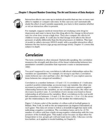
Figure 1-1 shows a plot of the number of coffees sold at football games in
Buffalo, New York, as well as the air temperature (in degrees Fahrenheit) at
each game. This data set seems to follow a downhill straight line fairly well,
indicating a negative correlation. The correlation turns out to be –0.741;
number of coffees sold has a fairly strong negative relationship with the tem-
perature of the football game. This makes sense because on days when the
temperature is low, people get cold and want more coffee. I discuss correla-
tion further, as it applies to model building, in Chapter 4.

05_466469-ch01.indd 17 7/24/09 9:30:48 AM