Page 65 - Statistics II for Dummies

Chapter 3: Reviewing Confidence Intervals and Hypothesis Tests
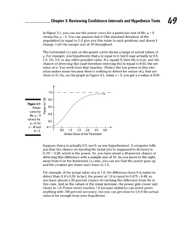
In Figure 3-1, you can see the power curve for a particular test of Ho: µ = 0 49
versus Ha: µ > 0. You can assume that σ (the standard deviation of the
population) is equal to 2 (I give you this value in each problem) and doesn’t
change. I set the sample size at 10 throughout.
The horizontal (x) axis on the power curve shows a range of actual values of
µ. For example, you hypothesize that µ is equal to 0, but it may actually be 0.5,
1.0, 2.0, 3.0, or any other possible value. If µ equals 0, then Ho is true, and the
chance of detecting this (and therefore rejecting Ho) is equal to 0.05, the set
value of α. You work from that baseline. (Notice the low power in this situ-
ation makes sense because there’s nothing to detect for values of µ that are
close to 0.) So, on the graph in Figure 3-1, when x = 0, you get a y-value of 0.05.

1.0

Figure 3-1: 0.8
Power Power (n=10) 0.6
curve for
Ho: µ = 0 0.4
versus Ha:
µ > 0, for 0.2
n = 10 and
σ = 2. 0.5 1.0 1.5 2.0 2.5 3.0
Actual Value of the Parameter

Suppose that µ is actually 0.5, not 0, as you hypothesized. A computer tells
you that the chance of rejecting Ho (what you’re supposed to do here) is
0.197 = 0.20, which is the power. So, you have about a 20-percent chance of
detecting this difference with a sample size of 10. As you move to the right,
away from 0 on the horizontal (x) axis, you can see that the power goes up
and the y-values get closer and closer to 1.0.

For example, if the actual value of µ is 1.0, the difference from 0 is easier to
detect than if it’s 0.50. In fact, the power at 1.0 is equal to 0.475 = 0.48, so
you have almost a 50 percent chance of catching the difference from Ho in
this case. And as the values of the mean increase, the power gets closer and
closer to 1.0. Power never reaches 1.0 because statistics can never prove
anything with 100 percent accuracy, but you can get close to 1.0 if the actual
value is far enough from your hypothesis.

7/23/09 9:23:27 PM
07_466469-ch03.indd 49 7/23/09 9:23:27 PM
07_466469-ch03.indd 49