Page 307 - Statistics for Dummies

Chapter 18: Looking for Links: Correlation and Regression
way, and sometimes not. This uncertainty differs from slope, which is always
interpretable. In fact, between the two elements of slope and y-intercept, the
slope is the star of the show, with the y-intercept serving as the less-famous
but still noticeable sidekick.
At times the y-intercept makes no sense. For example, suppose you use rain
to predict bushels per acre of corn. You know if the data set contains a point
where rain is 0, the bushels per acre must be 0 as well. As a result, if the
regression line crosses the y-axis somewhere else besides 0 (and there is no
guarantee it will cross at 0 — it depends on the data), the y-intercept will make
no sense. Similarly, in this context a negative value of y (corn production)
cannot be interpreted.
Another situation where you can’t interpret the y-intercept is when data are
not present near the point where x = 0. For example, suppose you want to
use students’ scores on Midterm 1 to predict their scores on Midterm 2. The
y-intercept represents a prediction for Midterm 2 when the score on Midterm
1 is 0. You don’t expect scores on a midterm to be at or near 0 unless some- 291
one didn’t take the exam, in which case her score wouldn’t be included in the
first place.
Many times, however, the y-intercept is of interest to you, it has meaning, and
you have data collected in the area where x = 0. For example, if you’re predict-
ing coffee sales at football games in Green Bay, Wisconsin, using temperature,
some games get cold enough to have temperatures at or even below 0 degrees
Fahrenheit, so predicting coffee sales at these temperatures makes sense. (As
you may guess, they sell more and more coffee as the temperature dips.)
Putting it all together with an example:
The regression line for the crickets
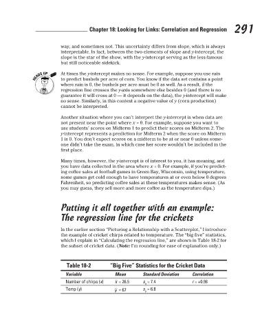
In the earlier section “Picturing a Relationship with a Scatterplot,” I introduce
the example of cricket chirps related to temperature. The “big five” statistics,
which I explain in “Calculating the regression line,” are shown in Table 18-2 for
the subset of cricket data. (Note: I’m rounding for ease of explanation only.)
Table 18-2 “Big Five” Statistics for the Cricket Data
Variable Mean Standard Deviation Correlation
Number of chirps (x) = 26.5 s = 7.4 r = +0.98
x
Temp (y) = 67 s = 6.8
y

3/25/11 8:13 PM
26_9780470911082-ch18.indd 291
26_9780470911082-ch18.indd 291 3/25/11 8:13 PM