Page 249 - Statistics for Environmental Engineers

L1592_frame_C28.fm Page 252 Tuesday, December 18, 2001 2:48 PM

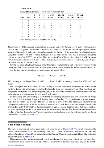
TABLE 28.4
4−1
Model Matrix for the 2 Fractional Factorial Design
==
1 2 3 4 == 123 12 == == 34 13 == == 24 23 == == 14
Run Avg. S D L F (SDL) SD (LF) SL (DF) DL (SF)
1 + − − − − + + +
2 + + − − + − − +
3 + − + − + − + −
4 + + + − − + − −
5 + − − + + + − −
6 + + − + − − + −
7 + − + + − − − +
8 + + + + + + + +
Note: Defining relation: I = 1234 (or I = SDLF).

Therefore, I = 1234 means that multiplying the column vectors for factors 1, 2, 3, and 4, which consists
of +1’s and −1’s, gives a vector that consists of +1 values. It also means that multiplying the column
vectors of factors 2, 3, and 4 gives the column vector for factor 1. This means that the effect calculated
using the column of +1 and −1 values for factor 1 is the same as the value that is calculated using the
column vector of the X 2 X 3 X 4 interaction. Thus, the main effect of factor 1 is confounded with the three-
factor interaction of factors 2, 3, and 4. Also, multiplying the column vectors of factors 1, 3, and 4 gives
the column vector for factor 2, etc.
Having the main effects confounded with three-factor interactions is part of the price we pay we to
investigate four factors in eight runs. Another price, which can be seen in the defining relation I = 1234,
is that the two-factor interactions are confounded with each other:

12 + 34 13 + 24 23 + 14

The two-way interaction of factors 1 and 2 is confounded with the two-way interaction of factors 3 and
4, etc.
The consequence of this intentional confounding is that the estimated main effects are biased unless
the three-factor interactions are negligible. Fortunately, three-way interactions are often small and can
be ignored. There is no safe basis for ignoring any of the two-factor interactions, so the effects calculated
as two-factor interactions must be interpreted with caution.
Understanding how confounding is identified by the defining relation reveals how the fractional design
was created. Any fractional design will involve some confounding. The experimental designer wants to
make this as painless as possible. The best we can do is to hope that the three-factor interactions are
unimportant and arrange for the main effects to be confounded with three-factor interactions. Intentionally
confounding factor 4 with the three-factor interaction of factors 1, 2, and 3 accomplishes that. By convention,
we write the design matrix in the usual form for the first three factors. The fourth column becomes the
product of the first three columns. Then we multiply pairs of columns to get the columns for the two-factor
interactions, as shown in Table 28.4.

Case Study Solution
The average response at each experimental setting is shown in Figure 28.1. The small boxes identify
the four tests that were conducted at the high flow rate (X 4 ); the low flow rate tests are the four unboxed
values. Calculation of the effects was explained in Chapter 27 and are not repeated here. The estimated
effects are given in Table 28.5.
This experiment has replication at each experimental condition so we can estimate the variance of the
measurement error and of the estimated effects. The differences between duplicates (d i ) can be used to
© 2002 By CRC Press LLC