Page 252 - Statistics for Environmental Engineers

L1592_frame_C28.fm Page 255 Tuesday, December 18, 2001 2:48 PM

TABLE 28.6
Constructing the Reference Distribution for Scale Factor =
0.82
t distribution (ν == == 8) Scaled Reference Distribution a
Value of t t Ordinate t ×× ×× 0.82 Ordinate/0.82
0 0.387 0.00 0.472
0.25 0.373 0.21 0.455
0.5 0.337 0.41 0.411
0.75 0.285 0.62 0.348
1.0 0.228 0.82 0.278
1.25 0.173 1.03 0.211
1.50 0.127 1.23 0.155
1.75 0.090 1.44 0.110
2.00 0.062 1.64 0.076
2.25 0.043 1.85 0.052
2.50 0.029 2.05 0.035
2.75 0.019 2.26 0.023
3.0 0.013 2.46 0.016
a
Scaling both the abscissa and the ordinate makes the area under the
reference distribution equal to 1.00.

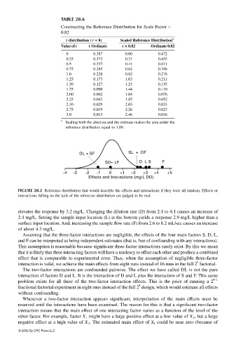
DL + SF SL + DF

SD+ LF D L S F
-4 -3 -2 -1 0 +1 +2 +3 +4 +5
Effects and Interactions (mg/L DO)

FIGURE 28.2 Reference distribution that would describe the effects and interactions if they were all random. Effects or
interactions falling on the tails of the reference distribution are judged to be real.

elevates the response by 3.2 mg/L. Changing the dilution rate (D) from 2:1 to 4:1 causes an increase of
2.4 mg/L. Setting the sample input location (L) at the bottom yields a response 2.9 mg/L higher than a
surface input location. And, increasing the sample flow rate (F) from 2.6 to 8.2 mL/sec causes an increase
of about 4.3 mg/L.
Assuming that the three-factor interactions are negligible, the effects of the four main factors S, D, L,
and F can be interpreted as being independent estimates (that is, free of confounding with any interactions).
This assumption is reasonable because significant three-factor interactions rarely exist. By this we mean
that it is likely that three interacting factors will have a tendency to offset each other and produce a combined
effect that is comparable to experimental error. Thus, when the assumption of negligible three-factor
4
interaction is valid, we achieve the main effects from eight runs instead of 16 runs in the full 2 factorial.
The two-factor interactions are confounded pairwise. The effect we have called DL is not the pure
interaction of factors D and L. It is the interaction of D and L plus the interaction of S and F. This same
problem exists for all three of the two-factor interaction effects. This is the price of running a 2 4−1
4
fractional factorial experiment in eight runs instead of the full 2 design, which would estimate all effects
without confounding.
Whenever a two-factor interaction appears significant, interpretation of the main effects must be
reserved until the interactions have been examined. The reason for this is that a significant two-factor
interaction means that the main effect of one interacting factor varies as a function of the level of the
other factor. For example, factor X 1 might have a large positive effect at a low value of X 2 , but a large
negative effect at a high value of X 2 . The estimated main effect of X 1 could be near zero (because of
© 2002 By CRC Press LLC