Page 66 - Sustainability in the Process Industry Integration and Optimization

Pro c ess O p timization 43

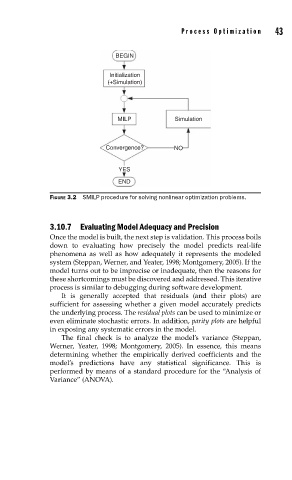
BEGIN

Initialization
(+Simulation)

MILP Simulation

Convergence? NO

YES
END
FIGURE 3.2 SMILP procedure for solving nonlinear optimization problems.

3.10.7 Evaluating Model Adequacy and Precision
Once the model is built, the next step is validation. This process boils
down to evaluating how precisely the model predicts real-life
phenomena as well as how adequately it represents the modeled
system (Steppan, Werner, and Yeater, 1998; Montgomery, 2005). If the
model turns out to be imprecise or inadequate, then the reasons for
these shortcomings must be discovered and addressed. This iterative
process is similar to debugging during software development.
It is generally accepted that residuals (and their plots) are
sufficient for assessing whether a given model accurately predicts
the underlying process. The residual plots can be used to minimize or
even eliminate stochastic errors. In addition, parity plots are helpful
in exposing any systematic errors in the model.
The final check is to analyze the model’s variance (Steppan,
Werner, Yeater, 1998; Montgomery, 2005). In essence, this means
determining whether the empirically derived coefficients and the
model’s predictions have any statistical significance. This is
performed by means of a standard procedure for the “Analysis of
Variance” (ANOVA).