Page 13 - The Geological Interpretation of Well Logs

- INTRODUCTION -

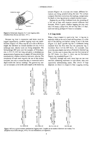
sensors (Figure |.4), so at any one instant, different for-
conducting cables
mations are being sampled along the tool, The surface
computer therefore memorizes the readings, compensates
for depth or time lag and gives a depth-matched output.
Despite the use of the combined tools, the recording of
a full set of logs still requires several different tool
malrix
descents. While a quick, shallow logging job may only
insulation
take 3-4 hours, a deep-hole, full set may take 2-3 days,
each tool taking perhaps 4-5 hours to complete.
steel support
Figure 1.3 Schematic diagram of a 7 core logging cable.
1.4 Log runs
(Modified from Moran and Attali, 1971.)
When a log is made it is said to be ‘run’. A sog run js
Because rig time is expensive and holes must be typically made at the end of each drilling phase, i.e. at the
logged immediately, modern logging tools are multi- end of the drilling and before casing is put in the hole
function (Figure 1.4). They may be up to 28 m (90 ft) in (Figure 1.5). Each specific log run is numbered, being
length, but still have an overall diameter of only 3-4 tn counted from the first time that the particular log is
(although new, shorter tools are being prepared). The recorded. Run 2 of the ISF Sonic, for example, may
Schlumberger ISF sonic too), for example, of 3%in diam- cover the same depth interval as a Formation Density Log
eter, is 55.5 ft (16.9 m) long and gives a simultaneous Run 1. in this case it means that over the first interval of
measurement of gamma ray or caliper, SP, deep resistivity the ISF Sonic, (i.e. Run 1), there was no Formation
(conductivity), shallow resistivity and sonic velocity. The Density log recorded (Figure 1.5).
complexity of such tools requires the use of the surface Typically, through any well, more logs are run over
computer, not only to record but also to memorize and to intervals containing reservoirs or with shows, than over
depth-match the various readings. The gamma-ray sen- apparently uninteresting zones. The choice of logs
sor, for example, is not at the same depth as the resistivity depends on what it is hoped to find. Logging costing
er 4
'
| I
3 = é. ~
. E> q §°
a Q
= at oe 14
€ o
E LU
a
a o
s|]& Si lg &
rae Sie _ 41 a
2 sii =~ sly a
alic
oO =
° io Tt1% «||
¢ nN
3 $| |e s1/&8 z/|s
3 o
¢ =
g 2 UD g
3 =
3a a
£ =f] --t3
IES-GR DIL-GR (ISF-GR
_- a
é. é
Es |. €
sonic sonic. S. & |
5 ('
5
-— 2
2 a
a-K| € _-lJ e eV le srg
ae N ce o
Pub fo 9 jis --)45 Lt 3
@ = =
2 = ~ a lA ~~
e| jz ig & | IS &
2 o z » 1
= 3 >» gx
eL|2 o lL & a 4 =
3. § 3s g
25 = eo |L 3
oa
S 2 4h
3 z
£ - =|
-- a J LY
OIL-SONIC-GR ISF-SONIC-GR DIL~Rxo-GNL-GR FOC-CNL-GR
Figure 1.4 Some typicai modern combination logging tools. Lengths are as marked; diameters are mainly 3 in.
(Modified from Schlumberger, 1974). For too] mnemonics see Appendix.
3