Page 260 - The Mechatronics Handbook

0066_frame_C12 Page 25 Wednesday, January 9, 2002 4:22 PM

n a
TABLE 12.5 Polytropic Processes: pv = Constant
General Ideal Gas b
(
p 2  n p 2  n  T 2 n/ n−1)
v 1
v 2
---- =  (1) ---- =  =  -----  (1′)
----
----
p 1 v 1 p 1 v 2 T 1
n = 0: constant pressure n = 0: constant pressure
n = ±∞: constant specific volume n = ±∞: constant specific volume
n = 1: constant temperature
n = k: constant specific entropy when k is constant
n = 1 n = 1
∫ 2 pv = p 1 v 1 ln v 2 (2) ∫ 2 pv = RT ln v 2 (2′)
----
----
d
d
1 v 1 1 v 1
----
----
– ∫ 2 vp = – p 1 v 1 ln p 2 (3) – ∫ 2 vp = – RT ln p 2 (3′)
d
d
1 p 1 1 p 1
n ≠ 1 n ≠ 1
(
∫ 2 pv = p 2 v 2 – p 1 v 1 ∫ 2 pv = RT 2 – T 1 )
--------------------------
-------------------------
d
d
1 1 – n ( 1 1 – n (
p 1 v 1
RT 1
p 2
p 2
= ------------ 1 –  n−1)/n (4) = ------------ 1 –  n−1)/n (4′)
----
----
n – 1  n – 1 
p 1
p 1
nR
n
d
d
– ∫ 2 vp = ------------ p 2 v 2 –( p 1 v 1 ) – ∫ 2 vp = ------------ T 2 –( T 1 )
1 1 – n 1 1 – n
= np 1 v 1  ( n−1)/n (5) = nRT 1  ( n−1)/n (5′)
p 2
p 2
------------- 1 –
------------- 1 –
----
----
n – 1  n – 1 
p 1
p 1
a
For polytropic processes of closed systems where volume change is the only work mode, Eqs. (2), (4), and
(2′), (4′) are applicable with Eq. (12.23) to evaluate the work. When each unit of mass passing through a one-inlet,
one-exit control volume at steady state undergoes a polytropic process, Eqs. (3), (5), and (3′), (5′) are applicable
2 2
–
with Eqs. (12.24a) and (12.24b) to evaluate the power. Also note that generally, ∫ 1 vdp = n∫ 1 pdv.
b
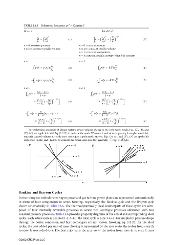
Rankine and Brayton Cycles
In their simplest embodiments vapor power and gas turbine power plants are represented conventionally
in terms of four components in series, forming, respectively, the Rankine cycle and the Brayton cycle
shown schematically in Table 12.6. The thermodynamically ideal counterparts of these cycles are com-
posed of four internally reversible processes in series: two isentropic processes alternated with two
constant pressure processes. Table 12.6 provides property diagrams of the actual and corresponding ideal
cycles. Each actual cycle is denoted 1-2-3-4-1; the ideal cycle is 1-2s-3-4s-1. For simplicity, pressure drops
through the boiler, condenser, and heat exchangers are not shown. Invoking Eq. (12.26) for the ideal
cycles, the heat added per unit of mass flowing is represented by the area under the isobar from state 2s
to state 3: area a-2s-3-b-a. The heat rejected is the area under the isobar from state 4s to state 1: area
©2002 CRC Press LLC