Page 810 - The Mechatronics Handbook

0066_Frame_C25 Page 9 Wednesday, January 9, 2002 7:05 PM

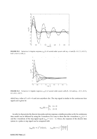
FIGURE 25.2 Variations in impulse response y imp (t) of second order system with ω n = 6 and β = 0.1( ), 0.2( ),
0.4(+), 0.6 ( * ), 0.8( ).

FIGURE 25.3 Variations in impulse response y imp (t) of second order system with β = 0.4 and ω n = 2( ), 4( ),
6(+), 8( * ), 10( ).

which has a value of 1 at k = 0 and zero anywhere else. The step signal is similar to the continuous time
signal and is given by

 0, k < 0
u step k() := 
 1, k ≥ 1

In order to characterize the discrete time pulse and step response a similar procedure as for the continuous
time model can be followed by using the z-transform. It is easy to show that the z-transform u imp (z) = 1
and the z-transform of the step signal equals u step z = z/(z − 1). Hence, the response of the discrete time
system to a pulse or step signal can be computed with

1 Gz()z 
– 
y imp k() = L { Gz()}, y step k() = L  -------------- 
1
–
–
 z 1 
©2002 CRC Press LLC