Page 958 - The Mechatronics Handbook

0066_Frame_C32.fm Page 8 Wednesday, January 9, 2002 7:54 PM

where
X = rectangular array (n + 1) × p,
n = number of inputs,
p = number of patterns.
Note that the size of the input patterns is always augmented by one, and this additional weight is responsible
for the threshold (see Fig. 32.3(b)). This method, similar to the LMS rule, assumes a linear activation
function, and so the net values net should be equal to desired output values d

Xw = d (32.16)

Usually p > n + 1, and the preceding equation can be solved only in the least mean square error sense.
Using the vector arithmetic, the solution is given by

1
–
T
T
w = ( X X) X d (32.17)
When traditional method is used, the set of p equations with n + 1 unknowns, Eq. (32.16), has to be
converted to the set of n + 1 equations with n + 1 unknowns
Yw = z (32.18)

where elements of the Y matrix and the z vector are given by

P P
y ij ∑ x ip x jp , z i ∑ x ip d p (32.19)
=
=
p=1 p=1
Weights are given by Eq. (32.17) or they can be obtained by a solution of Eq. (32.18).

Delta Learning Rule

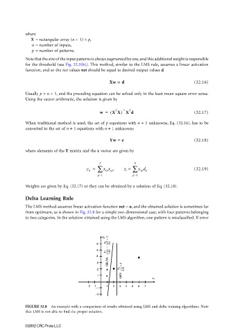
The LMS method assumes linear activation function net = o, and the obtained solution is sometimes far
from optimum, as is shown in Fig. 32.8 for a simple two-dimensional case, with four patterns belonging
to two categories. In the solution obtained using the LMS algorithm, one pattern is misclassified. If error

x 2 = 1
x 2
6 24
−
5
x 1 1.41
4
DELTA
3 = 1
2 x 1 2.5
LMS
1
x
1
−2 −1 1 2 3 4 5 6 7
−1
−2
FIGURE 32.8 An example with a comparison of results obtained using LMS and delta training algorithms. Note
that LMS is not able to find the proper solution.

©2002 CRC Press LLC