Page 960 - The Mechatronics Handbook

0066_Frame_C32.fm Page 10 Wednesday, January 9, 2002 7:54 PM

o 1
do k
A jk =
d net j
INPUTS x i w ij net j o k

o j OUTPUTS
jth
E j
+1

o K

+1

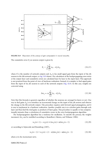
FIGURE 32.9 Illustration of the concept of gain computation in neural networks.

The cumulative error E j on neuron output is given by

K
1
E j = ---- ∑ ( o k – (32.27)
f j ′ d k )A jk
k=1
where K is the number of network outputs and A jk is the small signal gain from the input of the jth
neuron to the kth network output, as Fig. 32.9 shows. The calculation of the backpropagating error starts
at the output layer and cumulative errors are calculated layer by layer to the input layer. This approach
is not practical from the point of view of hardware realization. Instead, it is simpler to find signal gains
from the input of the jth neuron to each of the network outputs (Fig. 32.9). In this case, weights are
corrected using

K
∆w ij = cx i∑ ( o k – d k )A jk (32.28)
k=1

Note that this formula is general, regardless of whether the neurons are arranged in layers or not. One
way to find gains A jk is to introduce an incremental change on the input of the jth neuron and observe
the change in the kth network output. This procedure requires only forward signal propagation, and it
is easy to implement in a hardware realization. Another possible way is to calculate gains through each
layer and then find the total gains as products of layer gains. This procedure is equally or less computa-
tionally intensive than a calculation of cumulative errors in the error backpropagation algorithm.
The backpropagation algorithm has a tendency for oscillation. To smooth the process, the weights
increment ∆w ij can be modified according to Rumelhart, Hinton, and Wiliams (1986):

(
w ij n + 1) = w ij n() + ∆w ij n() + a∆w ij n 1) (32.29)
(
–
or according to Sejnowski and Rosenberg (1987),
(
w ij n +( 1) = w ij n() + ( 1 a)∆w ij n() + a∆w ij n 1) (32.30)
–
–
where a is the momentum term.

©2002 CRC Press LLC