Page 961 - The Mechatronics Handbook

0066_Frame_C32.fm Page 11 Wednesday, January 9, 2002 7:54 PM

f(net)
ACTUAL DERIVATIVE +1 OUTPUT

net
MODIFIED DERIVATIVE

DESIRED −1
OUTPUT

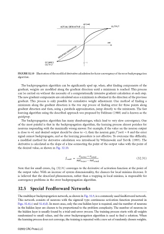
FIGURE 32.10 Illustration of the modified derivative calculation for faster convergency of the error backpropagation
algorithm.

The backpropagation algorithm can be significantly sped up, when, after finding components of the
gradient, weights are modified along the gradient direction until a minimum is reached. This process
can be carried on without the necessity of a computationally intensive gradient calculation at each step.
The new gradient components are calculated once a minimum is obtained in the direction of the previous
gradient. This process is only possible for cumulative weight adjustment. One method of finding a
minimum along the gradient direction is the tree step process of finding error for three points along
gradient direction and then, using a parabola approximation, jump directly to the minimum. The fast
learning algorithm using the described approach was proposed by Fahlman (1988) and is known as the
quickprop.
The backpropagation algorithm has many disadvantages, which lead to very slow convergency. One
of the most painful is that in the backpropagation algorithm, the learning process almost perishes for
neurons responding with the maximally wrong answer. For example, if the value on the neuron output
is close to +1 and desired output should be close to −1, then the neuron gain f ′(net) ≈ 0 and the error
signal cannot backpropagate, and so the learning procedure is not effective. To overcome this difficulty,
a modified method for derivative calculation was introduced by Wilamowski and Torvik (1993). The
derivative is calculated as the slope of a line connecting the point of the output value with the point of
the desired value, as shown in Fig. 32.10.

o desired – o actual
f modif = ---------------------------------------- (32.31)
net desired – net actual
Note that for small errors, Eq. (32.31) converges to the derivative of activation function at the point of
the output value. With an increase of system dimensionality, the chances for local minima decrease. It
is believed that the described phenomenon, rather than a trapping in local minima, is responsible for
convergency problems in the error backpropagation algorithm.

32.5 Special Feedforward Networks

The multilayer backpropagation network, as shown in Fig. 32.5, is a commonly used feedforward network.
This network consists of neurons with the sigmoid type continuous activation function presented in
Figs. 32.4(c) and 32.4(d). In most cases, only the one hidden layer is required, and the number of neurons
in the hidden layer are chosen to be proportional to the problem complexity. The number of neurons in
the hidden layer is usually found by a trial-and-error process. The training process starts with all weights
randomized to small values, and the error backpropagation algorithm is used to find a solution. When
the learning process does not converge, the training is repeated with a new set of randomly chosen weights.

©2002 CRC Press LLC