Page 966 - The Mechatronics Handbook

0066_Frame_C32.fm Page 16 Wednesday, January 9, 2002 7:54 PM

where
O = number of network outputs,
P = number of training patterns,
V p = output on the new hidden neuron,
E po = error on the network output.
V and E o are average values of V p and E po , respectively. By finding the gradient, dS/dw i , the weight,
adjustment for the new neuron can be found as

O P
∆w i ∑ ∑ s o E po – E o)f ′ p x ip (32.39)
(
=
o=1 p=1
where
s o = sign of the correlation between the new neuron output value and network output,
= derivative of activation function for pattern p,
f ′ p
x ip = input signal.
The output neurons are trained using the delta or quickprop algorithms. Each hidden neuron is trained
just once and then its weights are frozen. The network learning and building process is completed when
satisfactory results are obtained.

Radial Basis Function Networks

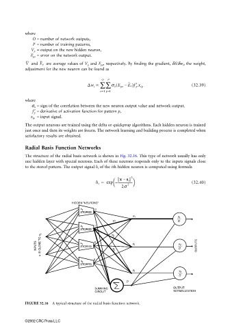
The structure of the radial basis network is shown in Fig. 32.16. This type of network usually has only
one hidden layer with special neurons. Each of these neurons responds only to the inputs signals close
to the stored pattern. The output signal h i of the ith hidden neuron is computed using formula

xs i 
–
h i = exp   – ------------------- 2 (32.40)
2 
2s

HIDDEN "NEURONS"
s 1 0
STORED
y 1
y 1
w 1 D
s 2 1
STORED w 2
x IS CLOSE TO s 2 s 3 0 y 2 y 2
INPUTS STORED w 3 D OUTPUTS

0
s 4
STORED
y 3
y 3
D
D
SUMMING OUTPUT
CIRCUIT NORMALIZATION

FIGURE 32.16 A typical structure of the radial basis function network.

©2002 CRC Press LLC