Page 175 - INTRODUCTION TO THE CALCULUS OF VARIATIONS

162 Isoperimetric inequality

R
R
A

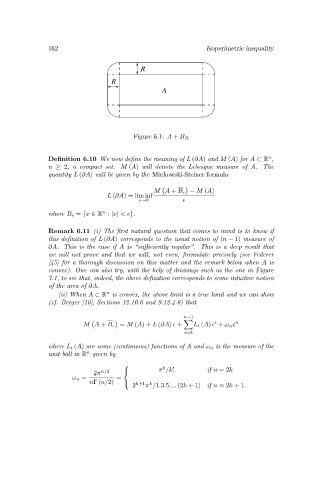
Figure 6.1: A + B R

n
Definition 6.10 We now define the meaning of L (∂A) and M (A) for A ⊂ R ,
n ≥ 2,a compact set. M (A) will denote the Lebesgue measure of A. The
quantity L (∂A) will be given by the Minkowski-Steiner formula

¡ ¢
M A + B − M (A)
L (∂A) = lim inf
→0
n
where B = {x ∈ R : |x| < }.

Remark 6.11 (i) The first natural question that comes to mind is to know if
this definition of L (∂A) corresponds to the usual notion of (n − 1) measure of
∂A. Thisisthe case if A is “sufficiently regular”. This is a deep result that
we will not prove and that we will, not even, formulate precisely (see Federer
[45] for a thorough discussion on this matter and the remark below when A is
convex). One can also try, with the help of drawings such as the one in Figure
7.1, to see that, indeed, the above definition corresponds to some intuitive notion
of the area of ∂A.
n
(ii) When A ⊂ R is convex, the above limit is a true limit and we can show
(cf. Berger [10], Sections 12.10.6 and 9.12.4.6) that
n−1
X
¡ ¢ i n
M A + B = M (A)+ L (∂A) + L i (A) + ω n
i=2
where L i (A) are some (continuous) functions of A and ω n is the measure of the
n
unit ball in R given by
⎧ k
π /k! if n =2k
n/2
⎨
2π
ω n = =
nΓ (n/2) ⎩ k+1 k
2 π /1.3.5.... (2k +1) if n =2k +1.