Page 250 - Thomson, William Tyrrell-Theory of Vibration with Applications-Taylor _ Francis (2010)

Sec. 8.2 Gauss Elimination 237

done by dividing the first row by 2.489 and adding it to the second row, which gives
"2.489 - 1 0 /O'
0 1.343 -1
0 - 1 0.7446
Although it is not necessary to go further in this case, the procedure can be
repeated to eliminate the - 1 term of the third row by dividing the second row by
1.343 and adding it to the third row, which results in
2.489 -1 0 l / x. \ ^' ^ / 0 \
1.343 - 1
0 0

In either this equation or the previous one, the amplitude is assigned the value
1, which results in the first eigenvector or mode:
( 1) ^0.2992^
0.7446
-
1 . 1.000 .
By repeating the procedure with A2 and A3, the eigenvectors for the second and
third modes can be found.
Eigenvectors can also be found by the method in Appendix C, p. 496.
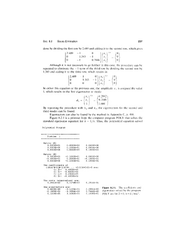
Figure 8.2-1 is a printout from the computer program POLY that solves the
standard eigenvalue equation for A = 1/A. Thus, the polynomial equation solved

Polynomial Program

Problem 1

Matrix [M]
0.2000E+01 O.OOOOE+00 O.OOOOE+00
O.OOOOE+00 O.lOOOE+01 O.OOOOE+00
O.OOOOE+00 O.OOOOE+00 O.lOOOE+01
Matrix [K]
0.3000E+01 -O.lOOOE+01 O.OOOOE+00
-O.lOOOE+01 0 .2000E+01 -O.lOOOE+01
O.OOOOE+00 -O.lOOOE+01 O.lOOOE+01
The coefficients of
C(N)X^N+C(N-1)X^N+ ... +C (1)X+C (0)=0 are:
C( 3)= O.lOOOE+01
C( 2)= -0.5000E+01
C( 1)= 0.4500E+01
C( 0)= -O.lOOOE+01
The roots (eigenvalues) are:
0.3461E+00 0.7378E+00 0.3916E+01
The eigenvectors are: Figure 8.2-1. The coefficients and
0.6800E+00 -0.1229E+01 0.2991E+00
-0.1889E+01 -0.3554E+00 0.7446E+00 eigenvalues solved by the program

O.lOOOE+01 O.lOOOE+01 O.lOOOE+01 POLY are for A= l/A = /c/mo;“.