Page 259 - Thomson, William Tyrrell-Theory of Vibration with Applications-Taylor _ Francis (2010)

246 Computational Methods Chap. 8

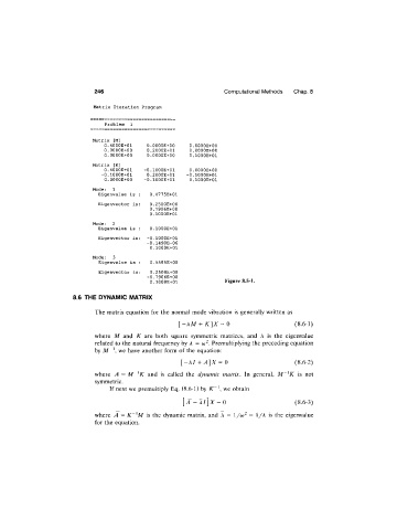
Matrix Iteration Program

Problem 1

Matrix [M]
0.4000E+01 O.OOOOE+00 O.OOOOE+00
O.OOOOE+00 0 .2000E+01 O.OOOOE+00
O.OOOOE+00 O.OOOOE+00 O.lOOOE+01
Matrix [K]
0.4000E+01 -O.lOOOE+01 0.OOOOE+00
-O.lOOOE+01 0 .2000E+01 -O.lOOOE+01
O.OOOOE+00 -O.lOOOE+01 O.lOOOE+01
Mode: 1
Eigenvalue is : 0.4775E+01
Eigenvector is: 0.2500E+00
0.7906E+00
O.lOOOE+01
Mode: 2
Eigenvalue is : O.lOOOE+01
Eigenvector is: -0.lOOOE+01
-0.1490E-06
O.lOOOE+01
Mode: 3
Eigenvalue is : 0.5585E+00
Eigenvector is: 0.2500E+00
-0.7906E+00
O.lOOOE+01 Figure 8.5-1.

8.6 THE DYNAMIC MATRIX

The matrix equation for the normal mode vibration is generally written as
[-AM + K ]X = 0 (8.6-1)

where M and K are both square symmetric matrices, and A is the eigenvalue

related to the natural frequency by A = Premultiplying the preceding equation
by M~^ we have another form of the equation;
[ ~ \ I + A ]X = 0 (8.6-2)
where A = M~^K and is called the dynamic matrix. In general, M~^K is not
symmetric.
If next we premultiply Eq. (8.6-1) by K~\ we obtain

A - k l \ X = 0 (8.6-3)

where A = K W is the dynamic matrix, and A = 1 /(d^ = 1/A is the eigenvalue
for the equation.