Page 301 - Thomson, William Tyrrell-Theory of Vibration with Applications-Taylor _ Francis (2010)

288 Vibration of Continuous Systems Chap. 9

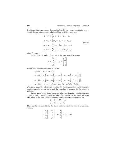
The Runge-K utta procedure, discussed in Sec. 4.6 for a single coordinate, is now
extended to the simultaneous solution of four variables listed next:

^ + -g-i/l + 2/2 + 2/3 +/4)

y + 2^2 + 2g3 + ^4)
(9.6-9)
M = Mj + 2/?2 + 2/?3 + P4)

V = + 2/C2 T 2/13 + /C4)
where /z = Ax.
Let /,, g,, p,, and T, G, F, and /C be represented by vectors
'f, \ iF
S,
k = L =
Pt
k:
Then the computation proceeds as follows:
= L(X|
( h r h h h h
12 = l [ x, 1 + 1 + /i^ > y> + P i 2 X i + k\2

, / h , h h .. , h
^3 = L lx , 1 + 2 ><Ai1 + /2 2 ’ >’1 + .^2'2 ’ "^1 + + k j j

= L (x j + /z, + f^h, yj + g^h, + k^^h)
With these quantities substituted into Eq. (9.6-9), the dependent variables at the
neighboring point X2 are found, and the procedure is repeated for the point X3,
and so on.
Let us return to the beam equations, where the boundary conditions at the
beginning end Xj provide a starting point. For example, in the cantilever beam
with origin at the fixed end, the boundary conditions at the starting end are
= 0, Mj = Mj
y, = 0, K, = K,
These can be considered to be the linear combination of two boundary vectors as
follows:
\
'•A, Í 0 ]
Í
yi 0 0

> = < > + ûf< >—G j + Of Z) j
M, 1 0
V,
0 , 1 ,