Page 370 - Thomson, William Tyrrell-Theory of Vibration with Applications-Taylor _ Francis (2010)

Sec. 11.3 Normal Modes of Constrained Structures 357

The slope-to-deflection ratio at jc = <3 is
y \ a ) D,(a>)
y (a)
^ E
D.(co)
The free-free mode shape is then given by

y { x )
= E

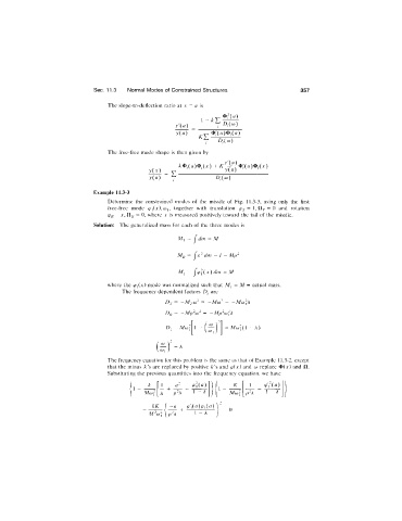
Example 11.3-3
Determine the constrained modes of the missile of Fig. 11.3-3, using only the first
free-free mode w,, together with translation l,ily = 0 and rotation
iP^ = X, = 0, where x is measured positively toward the tail of the missile.
f
Solution: The generalized mass for each of the three modes is

My - j dm = M

Mj^ = j d m = / = Mp^

M\ = j i p ] { x ) d m = M

where the (p,(x) mode was normalized such that = M ^ actual mass.
The frequency dependent factors D, arc
Dy = —Mj (o^ = —Mco^ = —M(jo\k

Df^ = —Mp^Ci)^ = —Mp^ia^A

(ii
D, = Mo) = Mia^( 1 —A)

(i) =A
—
The frequency equation for this problem is the same as that of Example 11.3-2, except
that the minus A’s arc replaced by positive A’s and (pix) and o) replace <I>(x) and O.
Substituting the previous quantities into the frequency equation, we have
k K

1 - 1 -

Mco] A p^A Miat p-k
kK -a ^ ip\{a)ip^{a)
I p^A = 0