Page 307 - Thermal Hydraulics Aspects of Liquid Metal Cooled Nuclear Reactors

Turbulent heat transport 277

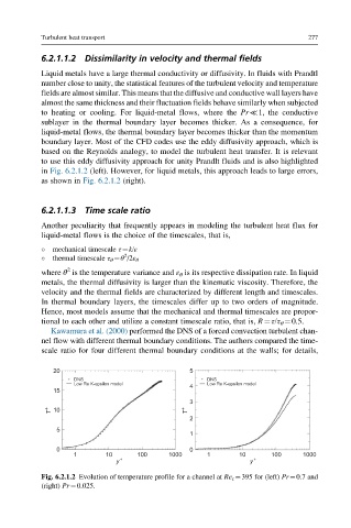
6.2.1.1.2 Dissimilarity in velocity and thermal fields

Liquid metals have a large thermal conductivity or diffusivity. In fluids with Prandtl
number close to unity, the statistical features of the turbulent velocity and temperature
fields are almost similar. This means that the diffusive and conductive wall layers have
almost the same thickness and their fluctuation fields behave similarly when subjected
to heating or cooling. For liquid-metal flows, where the Pr≪1, the conductive
sublayer in the thermal boundary layer becomes thicker. As a consequence, for
liquid-metal flows, the thermal boundary layer becomes thicker than the momentum
boundary layer. Most of the CFD codes use the eddy diffusivity approach, which is
based on the Reynolds analogy, to model the turbulent heat transfer. It is relevant
to use this eddy diffusivity approach for unity Prandlt fluids and is also highlighted
in Fig. 6.2.1.2 (left). However, for liquid metals, this approach leads to large errors,
as shown in Fig. 6.2.1.2 (right).

6.2.1.1.3 Time scale ratio
Another peculiarity that frequently appears in modeling the turbulent heat flux for
liquid-metal flows is the choice of the timescales, that is,
mechanical timescale τ¼k/ε
2
thermal timescale τ θ ¼θ /2ε θ
2
where θ is the temperature variance and ε θ is its respective dissipation rate. In liquid
metals, the thermal diffusivity is larger than the kinematic viscosity. Therefore, the
velocity and the thermal fields are characterized by different length and timescales.
In thermal boundary layers, the timescales differ up to two orders of magnitude.
Hence, most models assume that the mechanical and thermal timescales are propor-
tional to each other and utilize a constant timescale ratio, that is, R¼τ/τ θ ¼0.5.
Kawamura et al. (2000) performed the DNS of a forced convection turbulent chan-
nel flow with different thermal boundary conditions. The authors compared the time-
scale ratio for four different thermal boundary conditions at the walls; for details,

20 5
DNS DNS
Low Re K-epsilon model Low Re K-epsilon model
4
15
3
T + 10 T +
2
5
1
0 0
1 10 100 1000 1 10 100 1000
y + y +
Fig. 6.2.1.2 Evolution of temperature profile for a channel at Re τ ¼395 for (left) Pr¼0.7 and
(right) Pr¼0.025.