Page 103 - Bird R.B. Transport phenomena

88 Chapter 3 The Equations of Change for Isothermal Systems

We now turn to the illustrative examples. The first two are problems that were dis-
cussed in the preceding chapter; we rework these just to illustrate the use of the equa-
tions of change. Then we consider some other problems that would be difficult to set up
by the shell balance method of Chapter 2.

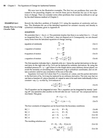
EXAMPLE 3.6-1 Rework the tube-flow problem of Example 2.3-1 using the equations of continuity and mo-
tion. This illustrates the use of the tabulated equations for constant viscosity and density in
Steady Flow in a Long cylindrical coordinates, given in Appendix B.
Circular Tube
SOLUTION
We postulate that v = b v {r, z). This postulate implies that there is no radial flow (v = 0) and
r
z
z
no tangential flow (v = 0), and that v does not depend on 0. Consequently, we can discard
e
z
many terms from the tabulated equations of change, leaving
equation of continuity (3.6-1)
r-equation of motion (3.6-2)

0-equation of motion 0 = - (3.6-3)
дв
z-equation of motion (3.6-4)

The first equation indicates that v depends only on r; hence the partial derivatives in the sec-
z
ond term on the right side of Eq. 3.6-4 can be replaced by ordinary derivatives. By using the
modified pressure & = p + pgh (where h is the height above some arbitrary datum plane), we
avoid the necessity of calculating the components of g in cylindrical coordinates, and we ob-
tain a solution valid for any orientation of the axis of the tube.
Equations 3.6-2 and 3.6-3 show that <3> is a function of z alone, and the partial derivative
in the first term of Eq. 3.6-4 may be replaced by an ordinary derivative. The only way that we
can have a function of r plus a function of z equal to zero is for each term individually to be a
constant—say, C —so that Eq. 3.6-4 reduces to
o
dv
(3.6-5)

The ty equation can be integrated at once. The ^-equation can be integrated by merely "peel-
ing off" one operation after another on the left side (do not "work out" the compound deriva-
tive there). This gives
9 = Qz + C, (3.6-6)

2
v z = ^ r + C In r + C 3 (3.6-7)
2
The four constants of integration can be found from the boundary conditions:
B.C.I at z = 0, (3.6-8)
B.C. 2 at z = L, (3.6-9)
B.C3 at r = R, (3.6-10)
B.C. 4 at r = 0, v 7 = finite (3.6-11)
The resulting solutions are:
(3.6-12)
P - <3> )R 2
o L
= • (3.6-13)
v 7
4/JLL