Page 116 - Bird R.B. Transport phenomena

§3.7 Dimensional Analysis of the Equations of Change 101

periment on a scale model of diameter D n = 1 ft. To have dynamic similarity, we must
choose conditions such that Re = Re^ Then if we use the same fluid in the small-scale
n
experiment as in the large system, so that /х /р п = Ц\/ p\, we find (IOH = 150 ft/s as the
f
п
required air velocity in the small-scale model. With the Reynolds numbers thus equal-
ized, the flow patterns in the model and the full-scale system will look alike: that is, they
are geometrically similar.
Furthermore, if Re is in the range of periodic vortex formation, the dimensionless
time interval t v^/D between vortices will be the same in the two systems. Thus, the vor-
v
tices will shed 25 times as fast in the model as in the full-scale system. The regularity of
4
2
the vortex shedding at Reynolds numbers from about 10 to 10 is utilized commercially
for precise flow metering in large pipelines.
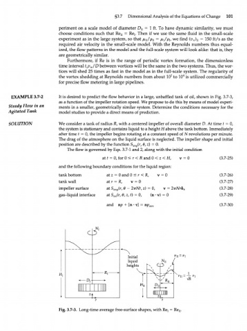
EXAMPLE 3.7-2 It is desired to predict the flow behavior in a large, unbaffled tank of oil, shown in Fig. 3.7-3,
as a function of the impeller rotation speed. We propose to do this by means of model experi-
Steady Flow in an ments in a smaller, geometrically similar system. Determine the conditions necessary for the
Agitated Tank model studies to provide a direct means of prediction.

SOLUTION We consider a tank of radius R, with a centered impeller of overall diameter D. At time t = 0,
the system is stationary and contains liquid to a height H above the tank bottom. Immediately
after time t = 0, the impeller begins rotating at a constant speed of N revolutions per minute.
The drag of the atmosphere on the liquid surface is neglected. The impeller shape and initial
position are described by the function S (r, 0, z) = 0.
imp
The flow is governed by Eqs. 3.7-1 and 2, along with the initial condition
at t = 0, for 0 < r < R and 0 < z < H, v = 0 (3.7-25)
and the following boundary conditions for the liquid region:
tank bottom at z = 0 and 0 < r < R, v = 0 (3.7-26)
tank wall at r = R, v = 0 (3.7-27)
impeller surface at S (r, в - 2тгМ, z) = 0, v = 2irNrb H (3.7-28)
imp
gas-liquid interface at S (r, 0, z, 0 = 0, (n • v) = 0 (3.7-29)
int
and np + [n • T] = np atm (3.7-30)

Fig. 3.7-3. Long-time average free-surface shapes, with Rej = Re .
n