Page 132 - Bird R.B. Transport phenomena

§4.1 Time-Dependent Flow of Newtonian Fluids 117

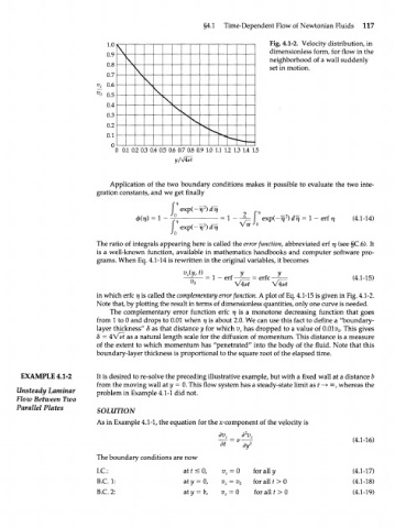
1.0 Fig. 4.1-2. Velocity distribution, in
\ dimensionless form, for flow in the
0.9
\ neighborhood of a wall suddenly
0.8 set in motion.
\
0.7
\
0.6
>
0.5
\
0.4
\
0.3
0.2
4
0.1
0
О 0.1 0.2 0.3 0.4 0.5 0.6 0.7 0.8 0.9 1.0 1.1 1.2 1.3 1.4 1.5

Application of the two boundary conditions makes it possible to evaluate the two inte-
gration constants, and we get finally
2
- )dr 1
v
(4.1-14)
J
2
exp(-i7 ; Vir o
J о
The ratio of integrals appearing here is called the error function, abbreviated erf r\ (see §C6). It
is a well-known function, available in mathematics handbooks and computer software pro-
grams. When Eq. 4.1-14 is rewritten in the original variables, it becomes
• = 1 - e r f - -. = erf с - (4.1-15)

in which erfc 17 is called the complementary error function. A plot of Eq. 4.1-15 is given in Fig. 4.1-2.
Note that, by plotting the result in terms of dimensionless quantities, only one curve is needed.
The complementary error function erfc 17 is a monotone decreasing function that goes
from 1 to 0 and drops to 0.01 when 17 is about 2.0. We can use this fact to define a "boundary-
layer thickness" 8 as that distance у for which v x has dropped to a value of 0.01 v . This gives
0
8 = \\/~vt as a natural length scale for the diffusion of momentum. This distance is a measure
of the extent to which momentum has "penetrated" into the body of the fluid. Note that this
boundary-layer thickness is proportional to the square root of the elapsed time.

EXAMPLE 4.1-2 It is desired to re-solve the preceding illustrative example, but with a fixed wall at a distance b
from the moving wall at у = 0. This flow system has a steady-state limit as t —> 00, whereas the
Unsteady Laminar problem in Example 4.1-1 did not.
Flow Between Two
Parallel Plates SOLUTION
As in Example 4.1-1, the equation for the x-component of the velocity is
dv д V x
(4.1-16)
x
The boundary conditions are now
I.C.: at t < 0, v = 0 for all у (4.1-17)
x
B.C.I: aty = 0, v = v for alH > 0 (4.1-18)
x 0
B.C. 2: aty = b, v x = 0 for alH > 0 (4.1-19)