Page 223 - Bird R.B. Transport phenomena

§7.5 Estimation of the Viscous Loss 207

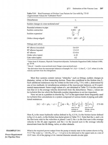
Table 7.5-1 Brief Summary of Friction Loss Factors for Use with Eq. 7.5-10
(Approximate Values for Turbulent Flow) fl

Disturbances e v
Sudden changes in cross-sectional area^
Rounded entrance to pipe 0.05
Sudden contraction 0.45(1 - j8)
Sudden expansion' - i

Orifice (sharp-edged) 2.71(1 -

Fittings and valves
90° elbows (rounded) 0.4-0.9
90° elbows (square) 1.3-1.9
45° elbows 0.3-0.4
Globe valve (open) 6-10
Gate valve (open) 0.2

a
Taken from H. Kramers, Physische Transportverschijnselen, Technische Hogeschool Delft, Holland (1958),
pp. 53-54.
b Here (3 = (smaller cross-sectional area)/(larger cross-sectional area).
c See derivation from the macroscopic balances in Example 7.6-1. If /3 = 0, then E = \{v) , where (v) is the
2
velocity upstream from the enlargement. v

Most flow systems contain various "obstacles," such as fittings, sudden changes in
diameter, valves, or flow measuring devices. These also contribute to the friction loss E .
v
Such additional resistances may be written in the form of Eq. 7.5-4, with e determined by
v
one of two methods: (a) simultaneous solution of the macroscopic balances, or (b) experi-
mental measurement. Some rough values of e are tabulated in Table 7.5-1 for the conven-
v
tion that (v) is the average velocity downstream from the disturbance. These e values are
v
for turbulent flow for which the Reynolds number dependence is not too important.
Now we are in a position to rewrite Eq. 7.4-7 in the approximate form frequently used
for turbulent flow calculations in a system composed of various kinds of piping and addi-
tional resistances:
2
M - v\) v f /) - lv e (7.5-10)
2
^h
sum over all /i sum over all
sections of fittings, valves,
straight conduits meters, etc.
Here R h is the mean hydraulic radius defined in Eq. 6.2-16,/is the friction factor defined
in Eq. 6.1-4, and e is the friction loss factor given in Table 7.5-1. Note that the v x and v 2 in
v
the first term refer to the velocities at planes 1 and 2; the v in the first sum is the average
velocity in the zth pipe segment; and the v in the second sum is the average velocity
downstream from the zth fitting, valve, or other obstacle.

EXAMPLE 7.5-1 What is the required power output from the pump at steady state in the system shown in Fig.
7.5-1? The water (p = 62.4 lb /ft ; /л = 1.0 cp) is to be delivered to the upper tank at a rate of
3
w
Power Requirement 12 ft /min. All of the piping is 4-in. internal diameter smooth circular pipe.
3
for Pipeline Flow