Page 225 - Bird R.B. Transport phenomena

§7.6 Use of the Macroscopic Balances for Steady-State Problems 209

Table 7.6-1 Steady-State Macroscopic Balances for Turbulent Flow in Isothermal Systems
Mass: (A)
Momentum: 2(z>]к», + S,)u, - 2( Р2И 2 2 2 + m tot g == F ^ (B)
Pl
; + p S )u 2
Angular momentum: 2(z>,w, + p,S,)[r, x u,] - X(v u ^2 + Р2^2)[Г 2 X u 2 ] + T ex t = T f .^ (C)
2
Mechanical energy: 2 E B (D)

Notes:
(a) All formulas here assume flat velocity profiles.
+ . . , where г<? 1я = p le u lfl S lfl/ etc.
.
(b) Sw 2 = w ]n + zv w + w lc
(c) h x and /z 2 are elevations above an arbitrary datum plane.
(d) All equations are written for compressible flow; for incompressible flow, E c = 0.
§7.6 USE OF THE MACROSCOPIC BALANCES
FOR STEADY-STATE PROBLEMS
In §3.6 we saw how to set up the differential equations to calculate the velocity and pres-
sure profiles for isothermal flow systems by simplifying the equations of change. In this
section we show how to use the set of steady-state macroscopic balances to obtain the al-
gebraic equations for describing large systems.
For each problem we start with the four macroscopic balances. By keeping track of
the discarded or approximated terms, we automatically have a complete listing of the as-
sumptions inherent in the final result. All of the examples given here are for isothermal,
incompressible flow. The incompressibility assumption means that the velocity of the
fluid must be less than the velocity of sound in the fluid and the pressure changes must
be small enough that the resulting density changes can be neglected.
The steady-state macroscopic balances may be easily generalized for systems with
multiple inlet streams (called la, lb, lc,...) and multiple outlet streams (called 2a, 2b,
2c,...). These balances are summarized in Table 7.6-1 for turbulent flow (where the ve-
locity profiles are regarded as flat).

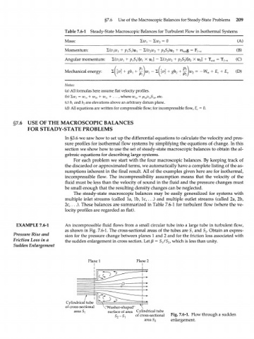
EXAMPLE 7.6-1 An incompressible fluid flows from a small circular tube into a large tube in turbulent flow,
as shown in Fig. 7.6-1. The cross-sectional areas of the tubes are S-y and S . Obtain an expres-
2
Pressure Rise and sion for the pressure change between planes 1 and 2 and for the friction loss associated with
Friction Loss in a the sudden enlargement in cross section. Let /3 = Si/S , which is less than unity.
Sudden Enlargement 2

Plane 1 Plane 2
I

Cylindrical tube
of cross-sectional V'Washer-shaped" \
surface of area Cylindrical tube
S - Si of cross-sectional Fig. 7.6-1. Flow through a sudden
2
area S 2 enlargement.