Page 231 - Bird R.B. Transport phenomena

§7.6 Use of the Macroscopic Balances for Steady-State Problems 215

or
-^ (V 2a w 2a ~ V 2h W 2b ) (7.6-36)

Now Eqs. 7.6-31, 32, 33, and 36 are four equations with four unknowns. When these are
solved we find that

= \w^(l + cos 0)
v 2a = v x w 2a (7.6-37, 38)
= г?, = Iw^l - cos 6)
v 2b w 2h (7.6-39,40)
Hence the velocities of all three streams are equal. The same result is obtained by applying
the classical Bernoulli equation for the flow of an inviscid fluid (see Example 3.5-1).

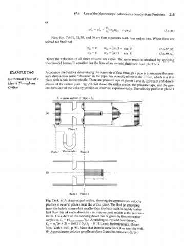
EXAMPLE 7.6-5 A common method for determining the mass rate of flow through a pipe is to measure the pres-
sure drop across some "obstacle" in the pipe. An example of this is the orifice, which is a thin
Isothermal Flow of a plate with a hole in the middle. There are pressure taps at planes 1 and 2, upstream and down-
Liquid Through an stream of the orifice plate. Fig. 7.6-5(я) shows the orifice meter, the pressure taps, and the gen-
Orifice eral behavior of the velocity profiles as observed experimentally. The velocity profile at plane 1

= cross section of pipe = S 2

(a)

Plane 1 Manometer P l a n e 2

(b)

I U
I I
I I
Plane 0 Plane 2
Fig. 7.6-5. (a)A sharp-edged orifice, showing the approximate velocity
profiles at several planes near the orifice plate. The fluid jet emerging
from the hole is somewhat smaller than the hole itself. In highly turbu-
lent flow this jet necks down to a minimum cross section at the vena con-
tracta. The extent of this necking down can be given by the contraction
coefficient, C = (S venacontracta /S ). According to inviscid flow theory,
0
c
C c = 7T/(T7 + 2) = 0.611 if SQ/ST = 0 [H. Lamb, Hydrodynamics, Dover,
New York (1945), p. 99]. Note that there is some back flow near the wall.
(b) Approximate velocity profile at plane 2 used to estimate {v\)/(v ).
2