Page 404 - Bird R.B. Transport phenomena

386 Chapter 12 Temperature Distributions with More Than One Independent Variable

For every complex function w{z), two heat flow nets are obtained by interchanging
the lines of constant / and the lines of constant g. Furthermore, two additional nets are
obtained by working with the inverse function z(w) as illustrated in Chapter 4 for ideal
fluid flow.
Note that potential fluid flow and potential heat flow are mathematically similar, the
two-dimensional flow nets in both cases being described by analytic functions. Physi-
cally, however, there are certain important differences. The fluid flow nets described in
§4.3 are for a fluid with no viscosity (a fictitious fluid!), and therefore one cannot use
them to calculate the drag forces at surfaces. On the other hand, the heat flow nets de-
scribed here are for solids that have a finite thermal conductivity, and therefore the re-
sults can be used to calculate the heat flow at all surfaces. Moreover, in §4.3 the velocity
profiles do not satisfy the Laplace equation, whereas in this section the temperature pro-
files do satisfy the Laplace equation. Further information about analogous physical
processes described by the Laplace equation is available in books on partial differential
equations. 3
Here we give just one example to provide a glimpse of the use of analytic functions;
further examples may be found in the references cited.

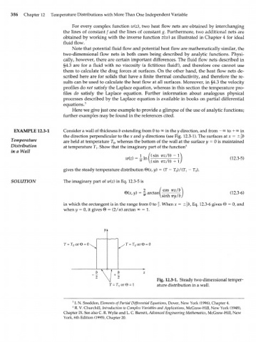
EXAMPLE 12.3-1 Consider a wall of thickness b extending from 0 to °o in the у direction, and from - °° to + °o in
the direction perpendicular to the x and у directions (see Fig. 12.3-1). The surfaces at x = ±\b
Temperature are held at temperature T , whereas the bottom of the wall at the surface у = 0 is maintained
o
Distribution at temperature T Show that the imaginary part of the function 4
in a Wall v
1 . /(sin irz/b) - 1
(12.3-5)
gives the steady temperature distribution ©(*, y) = (T - T )/(T } - T ).
o
0
SOLUTION The imaginary part of w(z) in Eq. 12.3-5 is

гч/ ч 2 ( COS 7TX/b\ /-,o-w4
©(*, v) = ^ arctan — — (12.3-6)
\sinh iry/b)
J w
in which the arctangent is in the range from 0 to f. When x = ±\b, Eq. 12.3-6 gives © = 0, and
when у = 0, it gives © = (2/тг) arctan °° = 1.

T = T o or 0 = 0 s T=T 0 orQ =

Fig. 12.3-1. Steady two-dimensional temper-
T = 7\ or 0 = 1 ature distribution in a wall

1. N. Sneddon, Elements of Partial Differential Equations, Dover, New York (1996), Chapter 4.
3
R. V. Churchill, Introduction to Complex Variables and Applications, McGraw-Hill, New York (1948),
4
Chapter IX. See also C. R. Wylie and L. C. Barrett, Advanced Engineering Mathematics, McGraw-Hill, New
York, 6th Edition (1995), Chapter 20.