Page 407 - Bird R.B. Transport phenomena

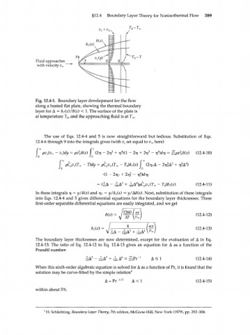
§12.4 Boundary Layer Theory for Nonisothermal Flow 389

Fluid approaches
with velocity v^

Fig. 12.4-lc Boundary layer development for the flow
along a heated flat plate, showing the thermal boundary
layer for A = 8 (x)/8(x) < 1. The surface of the plate is
T
at temperature T , and the approaching fluid is at Т .
ж
o
The use of Eqs. 12.4-4 and 5 is now straightforward but tedious. Substitution of Eqs.
12.4-6 through 9 into the integrals gives (with v set equal to v x here)
e
v
f pv (v x - )dy = vl8(x) Г' (2T7 - 2 V 3 (12.4-10)
x
x
P
Jo Jo
- T)dy = pC vJJ» - T )8 (x)
p 0 T
3
•(1 - 2 VT + 2 V T
- T )8 (x) (12.4-11)
0
T
In these integrals 17 = y/8(x) and r/ 7 = y/8 (x) = y/A5(x). Next, substitution of these integrals
T
into Eqs. 12.4-4 and 5 gives differential equations for the boundary layer thicknesses. These
first-order separable differential equations are easily integrated, and we get
1260
(12.4-12)

8 (x) = (12.4-13)
T 3
^A - TIHA + T^
The boundary layer thicknesses are now determined, except for the evaluation of A in Eq.
12.4-13. The ratio of Eq. 12.4-12 to Eq. 12.4-13 gives an equation for A as a function of the
Prandtl number:
-A 3 - —A 5 4- — A 6 = —Pr" 1 A < 1 (12.4-14)
15^* 140^* ^ 180 ^ 315 1 Г 1А — L
When this sixth-order algebraic equation is solved for A as a function of Pr, it is found that the
solution may be curve-fitted by the simple relation 4
(12.4-15)

within about 5%.

H. Schlichting, Boundary-Layer Theory, 7th edition, McGraw-Hill, New York (1979), pp. 292-308.
4