Page 410 - Bird R.B. Transport phenomena

392 Chapter 12 Temperature Distributions with More Than One Independent Variable

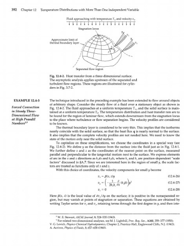
Fluid approaching with temperature T^ and velocity v^
ТТТТТТТТТГТТТТТТТТ
Stagnation locus

Approximate limit of
thermal boundary layer

Separated flow region

Fig. 12.4-2. Heat transfer from a three-dimensional surface.
The asymptotic analysis applies upstream of the separated and
turbulent flow regions. These regions are illustrated for cylin-
ders in Fig. 3.7-2.

EXAMPLE 12.4-3 The technique introduced in the preceding example has been extended to flow around objects
of arbitrary shape. Consider the steady flow of a fluid over a stationary object as shown in
Forced Convection Fig. 12.4-2. The fluid approaches at a uniform temperature T , and the solid surface is main-
x
in Steady Three- tained at a uniform temperature T . The temperature distribution and heat transfer rate are to
o
Dimensional Flow be found for the region of laminar flow, which extends downstream from the stagnation locus
at High Prandtl to the place where turbulence or flow separation begins. The velocity profiles are considered
Numbers 89 to be known.
The thermal boundary layer is considered to be very thin. This implies that the isotherms
nearly coincide with the solid surface, so that the heat flux q is nearly normal to the surface.
It also implies that the complete velocity profiles are not needed here. We need to know the
state of the motion only near the solid surface.
To capitalize on these simplifications, we choose the coordinates in a special way (see
Fig. 12.4-2). We define у as the distance from the surface into the fluid just as in Fig. 12.4-1.
We further define x and z as the coordinates of the nearest point on the surface, measured
parallel and perpendicular to the tangential motion next to the surface. We express elements
of arc in the x and z directions as h dx and h dz, where h and h are position-dependent "scale
x
z
x
z
factors" discussed in §A.7. Since we are interested here in the region of small y, the scale fac-
tors are treated as functions only of x and z.
With this choice of coordinates, the velocity components for small у become
v x = x, z)y (12.4-26)
(12.4-27)
i
2h x h z
(12.4-28)
Here /3(x, z) is the local value of dv /dy on the surface; it is positive in the nonseparated re-
x
gion, but may vanish at points of stagnation or separation. These equations are obtained by
writing Taylor series for v and v , retaining terms through the first degree in y, and then inte-
x
z
8
W. E. Stewart, AlChE Journal, 9, 528-535 (1963).
9
For related two-dimensional analyses, see M. J. Lighthill, Proc. Roy. Soc, A202, 359-377 (1950);
V. G. Levich, Physico-Chemical Hydrodynamics, Chapter 2, Prentice-Hall, Englewood Cliffs, N.J. (1962);
A. Acrivos, Physics of Fluids, 3, 657-658 (1960).