Page 652 - Bird R.B. Transport phenomena

632 Chapter 20 Concentration Distributions with More Than One Independent Variable

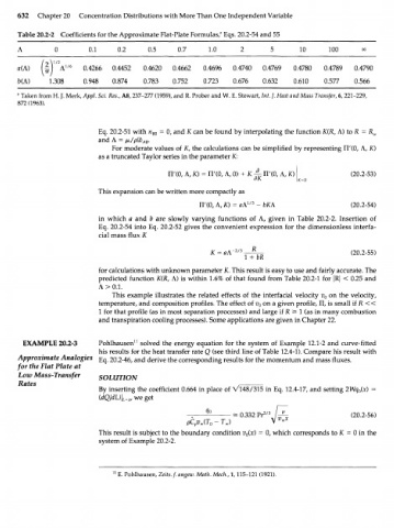
Table 20.2-2 Coefficients for the Approximate Flat-Plate Formulas/ Eqs. 20.2-54 and 55
л 0 0.1 0.2 0.5 0.7 1.0 2 5 10 100 00

я(Л) 0.4266 0.4452 0.4620 0.4662 0.4696 0.4740 0.4769 0.4780 0.4789 0.4790
НА) 1.308 0.948 0.874 0.783 0.752 0.723 0.676 0.632 0.610 0.577 0.566

" Taken from H. J. Merk, Appl. Sci. Res., A8, 237-277 (1959), and R. Prober and W. E. Stewart, Int. ]. Heat and Mass Transfer, 6, 221-229,
872 (1963).

Eq. 20.2-51 with n = 0, and К can be found by interpolating the function K(R, A) to R = R
B0 w
and Л = /л/рЯЬ .
АВ
For moderate values of K, the calculations can be simplified by representing П'(0, Л, К)
as a truncated Taylor series in the parameter K:
П'(0, Л, К) = П'(0, Л, 0) + К ^ П'(0, Л, К) (20.2-53)

This expansion can be written more compactly as
1/3
П'(0, А, К) = яЛ - ЬКА (20.2-54)
in which a and b are slowly varying functions of A, given in Table 20.2-2. Insertion of
Eq. 20.2-54 into Eq. 20.2-52 gives the convenient expression for the dimensionless interfa-
cial mass flux К

2/3
К = аА- —^— (20.2-55)
for calculations with unknown parameter K. This result is easy to use and fairly accurate. The
predicted function K(R, A) is within 1.6% of that found from Table 20.2-1 for |R| < 0.25 and

This example illustrates the related effects of the interfacial velocity v 0 on the velocity,
temperature, and composition profiles. The effect of v 0 on a given profile, П, is small if R «
1 for that profile (as in most separation processes) and large if R > 1 (as in many combustion
and transpiration cooling processes). Some applications are given in Chapter 22.

EXAMPLE 20.2-3 Pohlhausen 11 solved the energy equation for the system of Example 12.1-2 and curve-fitted
his results for the heat transfer rate Q (see third line of Table 12.4-1). Compare his result with
Approximate Analogies щ 20.2-46, and derive the corresponding results for the momentum and mass fluxes.
for the Flat Plate at
Low Mass-Transfer SOLUTION
Rates ,
By inserting the coefficient 0.664 in place of VI48/315 in Eq. 12.4-17, and setting 2Wq (x) =
o
(dQ/dL)\ L=x , we get
— = 0.332 Pr 2/3 / ^ (20.2-56)

This result is subject to the boundary condition v (x) = 0, which corresponds to К = 0 in the
o
system of Example 20.2-2.

1
E. Pohlhausen, Zeits.f. angew. Math. Mech., 1,115-121 (1921).