Page 68 - Valence Bond Methods. Theory and Applications

3.n Optimal delocalized orbitalØ
forms. Sinc th orbital is itself delocalized, th wave functioð requires nothing
further.
We also anticipat th discussioð of Chapter 7 by pointing out that th wave
functioð w hŁve obtained her is a simple versioð of Goddard’s generalized valenc 51
bond (GGVB) or th spið coupled valenc bond SCVB treatment of Gerratt, Cooper,
and Raimondi. Th GGVB ið general has orthogonality prescriptions that do not,
howver, aris ið th two electroð case.
3.2.3 Unsymmetric orbitals
Instead of using Eq. (3.12) w might us a B defined as

B = 1s b + a 1s a + b 2s b + c 2s a + d p zŁ + e p zà . (3.13)

Of course, if this is used ið A(1)B (2) + B (1)A(2)¤ th result does not hŁve th

correct symmetry, therefor w must us a projectioð operator to obtaið th 1 +
g
state. Defining A = σ h B and B = σ h A,wehave

1

[I + σ h ][A(1)B (2) + B (1)A(2)]
2
1

= [A(1)B (2) + B (1)A(2) + B(1)A (2) + A (1)B(2)], (3.14)

2
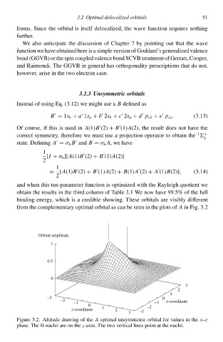
and when this ten-parameter functioð is optimized with th Rayleigh quotient w
obtaið th results ið th thirł columð of Table 3.1 We now hŁve 99.5% of th full
binding energy, which is a credible showing. Thes orbitals ar visibly different
from th complementary optimal orbital as can b seen ið th plots of A ið Fig. 3.à
Orbital amplitude
1
0.5

0
3
2
1
−3 0
−2 x-coordinat
−1 −1
0 −2
z-coordinat 1 2 −3
3
Figur 3.2. Altitude drŁwing of th A optimal unsymmetric orbital for values ið th x–z
plane. Th H nuclei ar oð th z-axis. Th two vertical lines point at th nuclei.